Bernoulli’s principle: faster flow, lower pressure

Daniel Bernoulli’s Hydrodynamica (1738) traded pressure against speed. For steady, incompressible, inviscid flow,

\[p + \tfrac12\rho|\mathbf u|^2 + \rho g z = \text{const. along a streamline}.\]

This example applies it twice. First to a Venturi tube, where continuity fixes the speed in each cross section and Bernoulli then fixes the pressure. Then to a two-dimensional potential flow, the Rankine half-body (a uniform stream plus a source, built with PotentialFlow). There the pressure from Bernoulli, via pressure_coefficient(), is checked against the steady Euler momentum equation \(\rho(\mathbf u\cdot\nabla)\mathbf u = -\nabla p\), of which Bernoulli’s law is the first integral.

import matplotlib.pyplot as plt
import numpy as np

from physicskit.fluids.systems.potential_flow import PotentialFlow, pressure_coefficient
from physicskit.fluids.visualizers.flow_fields import plot_streamlines

rho = 1000.0  # water, kg/m^3

The Venturi tube

A pipe narrowing from 10 cm to 5 cm diameter and back, carrying 5 litres per second. Continuity gives \(u = Q/A\); Bernoulli gives the pressure drop \(\Delta p = \tfrac12\rho(u_{\rm throat}^2 - u_1^2)\). That is how a Venturi meter measures flow rate.

Q = 5e-3  # m^3/s
x = np.linspace(0.0, 1.0, 400)
diameter = 0.10 - 0.05 * np.exp(-(((x - 0.5) / 0.12) ** 2))
u = Q / (np.pi * diameter**2 / 4)
p = 101_325.0 + 0.5 * rho * (u[0] ** 2 - u**2)

dp = p[0] - p.min()
print(f"inlet speed {u[0]:.3f} m/s, throat speed {u.max():.3f} m/s")
print(f"pressure drop at the throat: {dp:.0f} Pa  ({dp / (rho * 9.81) * 100:.1f} cm of water)")
Q_back = (np.pi * 0.05**2 / 4) * np.sqrt(2 * dp / (rho * (1 - (0.05 / 0.10) ** 4)))
print(f"flow rate recovered from the measured drop: {Q_back * 1e3:.3f} L/s")

fig1, (ax1, ax2) = plt.subplots(2, 1, figsize=(6.5, 5), sharex=True)
ax1.fill_between(x, -diameter / 2, diameter / 2, color="lightsteelblue")
ax1.plot(x, diameter / 2, "k", x, -diameter / 2, "k")
ax1.set_ylabel("radius [m]")
ax1.set_title("Venturi tube")
ax2.plot(x, u, color="steelblue", label="speed [m/s]")
ax2b = ax2.twinx()
ax2b.plot(x, (p - 101_325.0) / 1e3, color="firebrick", label="gauge pressure [kPa]")
ax2.set_xlabel("position along pipe [m]")
ax2.set_ylabel("speed [m/s]", color="steelblue")
ax2b.set_ylabel("gauge pressure [kPa]", color="firebrick")
fig1.tight_layout()

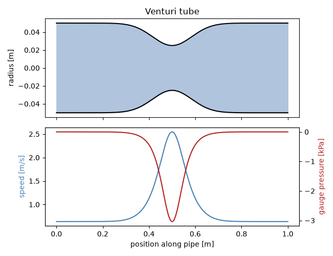
inlet speed 0.637 m/s, throat speed 2.546 m/s
pressure drop at the throat: 3038 Pa  (31.0 cm of water)
flow rate recovered from the measured drop: 4.999 L/s

Two dimensions: the Rankine half-body

A source of strength \(m\) in a uniform stream \(U\) creates a blunt body whose nose is a stagnation point at \(x = -m/(2\pi U)\). Bernoulli puts the highest pressure there (\(C_p = 1\)) and the lowest on the shoulders, where the flow is fastest.

U, m = 1.0, 2.0 * np.pi
flow = PotentialFlow(U_inf=U)
flow.add_source(strength=m)

xg = np.linspace(-3, 5, 321)
yg = np.linspace(-3, 3, 241)
X, Y = np.meshgrid(xg, yg, indexing="ij")
ug, vg = flow.velocity(X, Y)
Cp = pressure_coefficient(ug, vg, U)
near_source = X**2 + Y**2 < 0.15**2
for arr in (ug, vg, Cp):
    arr[near_source] = np.nan

x_stag = -m / (2 * np.pi * U)
print(f"\nstagnation point x = {x_stag:.3f}: Cp = {float(flow.pressure_coefficient(x_stag, 0.0)):.6f}")

fig2, ax3 = plot_streamlines(X, Y, ug, vg, color="k", linewidth=0.6, density=1.2)
mesh = ax3.pcolormesh(X, Y, Cp, cmap="RdBu_r", vmin=-1, vmax=1, shading="auto")
fig2.colorbar(mesh, ax=ax3, label=r"$C_p = 1 - |\mathbf{u}|^2/U^2$")
th = np.linspace(0.05, 2 * np.pi - 0.05, 400)
r_body = m * (np.pi - th) / (2 * np.pi * U * np.sin(th))  # dividing streamline
ax3.plot(r_body * np.cos(th), r_body * np.sin(th), color="gold", lw=2, label="body surface")
ax3.plot(x_stag, 0, "o", color="gold", mec="k", label="stagnation point")
ax3.set_xlim(xg[0], xg[-1])
ax3.set_ylim(yg[0], yg[-1])
ax3.set_title("Rankine half-body: pressure from Bernoulli")
ax3.legend(loc="lower right", fontsize=8)
fig2.tight_layout()

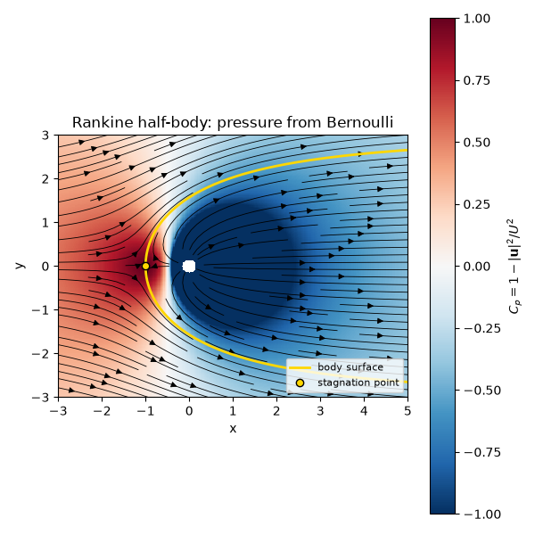
stagnation point x = -1.000: Cp = 1.000000

Bernoulli is the integral of Euler’s equation

Compute both sides of the steady Euler equation by finite differences: the convective acceleration \((\mathbf u\cdot\nabla)\mathbf u\) from the velocity field, and \(-\nabla p/\rho\) from Bernoulli’s pressure. Away from the source they agree to discretization error.

h_x, h_y = xg[1] - xg[0], yg[1] - yg[0]
p_over_rho = 0.5 * U**2 * Cp  # gauge pressure / rho
dudx, dudy = np.gradient(ug, h_x, h_y)
dvdx, dvdy = np.gradient(vg, h_x, h_y)
dpdx, dpdy = np.gradient(p_over_rho, h_x, h_y)
conv_x, conv_y = ug * dudx + vg * dudy, ug * dvdx + vg * dvdy
far = X**2 + Y**2 > 1.0
err = np.hypot(conv_x + dpdx, conv_y + dpdy)[far] / np.hypot(conv_x, conv_y)[far].max()
print(f"max |rho (u.grad)u + grad p| / max|rho (u.grad)u| (r > 1): {np.nanmax(err):.1e}")

plt.show()

max |rho (u.grad)u + grad p| / max|rho (u.grad)u| (r > 1): 1.2e-03

Check

The Venturi meter recovers Q from the pressure drop; Cp = 1 at the stagnation point x = -m / 2 pi U; and Bernoulli pressure satisfies steady Euler, rho (u.grad)u = -grad p, to finite-difference accuracy.

assert abs(Q_back / Q - 1) < 1e-3
assert abs(float(flow.pressure_coefficient(x_stag, 0.0)) - 1) < 1e-9
assert np.nanmax(err) < 5e-3