Co-rotating pair versus translating dipole

An isolated point vortex of circulation \(\Gamma\) induces a purely azimuthal velocity of magnitude \(\Gamma/(2\pi r)\) at distance r (the 2D Biot-Savart law); for two vortices separated by distance \(d\), this is exactly the speed each one advects with, carried by the field of the other. What the pair then does depends only on the relative sign of their circulation. Equal circulations \(\Gamma\) each orbit the common midpoint at radius \(d/2\), so their induced speed \(\Gamma/(2\pi d)\) translates into a rigid-body angular velocity

\[\Omega = \frac{\Gamma/(2\pi d)}{d/2} = \frac{\Gamma}{\pi d^2}.\]

Opposite circulations \(\pm\Gamma\) instead induce velocity in the same direction on each other (a “vortex dipole”), so the pair self-propels together in a straight line at constant speed

\[v = \frac{\Gamma}{2\pi d},\]

perpendicular to the line joining them, advecting each other sideways forever rather than orbiting. Both trajectories come from exactly the same PointVortexSystem – only the sign of one circulation changes between them.

import matplotlib.pyplot as plt
import numpy as np

from physicskit.fluids.systems.vortex_dynamics import PointVortexSystem
from physicskit.fluids.visualizers import theme

A co-rotating pair

Equal circulations orbit their midpoint at angular velocity \(\Omega = \Gamma / (\pi d^2)\).

Gamma, d = 1.0, 1.0
pair = PointVortexSystem(positions=[[d / 2, 0.0], [-d / 2, 0.0]], circulations=[Gamma, Gamma])
period = 2 * np.pi / (Gamma / (np.pi * d**2))
_, trajectory_pair = pair.trajectory(dt=period / 2000, n_steps=2000)

A translating dipole

Equal and opposite circulations instead translate together at constant speed \(\Gamma / (2\pi d)\), perpendicular to the line joining them.

dipole = PointVortexSystem(positions=[[0.0, d / 2], [0.0, -d / 2]], circulations=[Gamma, -Gamma])
travel_time = 4.0 * d / (Gamma / (2 * np.pi * d))
_, trajectory_dipole = dipole.trajectory(dt=travel_time / 2000, n_steps=2000)

Plot both trajectories

fig, axes = plt.subplots(1, 2, figsize=(11, 5))
axes[0].plot(trajectory_pair[:, 0, 0], trajectory_pair[:, 0, 1], color=theme.PRIMARY, label="vortex 1")
axes[0].plot(trajectory_pair[:, 1, 0], trajectory_pair[:, 1, 1], color=theme.ACCENT, label="vortex 2")
axes[0].set_aspect("equal")
axes[0].set_title("Co-rotating pair (same sign): rigid orbit")
axes[0].legend()

axes[1].plot(trajectory_dipole[:, 0, 0], trajectory_dipole[:, 0, 1], color=theme.PRIMARY, label="vortex 1")
axes[1].plot(trajectory_dipole[:, 1, 0], trajectory_dipole[:, 1, 1], color=theme.ACCENT, label="vortex 2")
axes[1].set_aspect("equal")
axes[1].set_title("Vortex dipole (opposite sign): self-propulsion")
axes[1].legend()
fig.tight_layout()

separation_pair = np.hypot(*(trajectory_pair[-1, 0] - trajectory_pair[-1, 1]).T)
separation_dipole = np.hypot(*(trajectory_dipole[-1, 0] - trajectory_dipole[-1, 1]).T)
print(f"pair separation: started at {d:.3f}, ended at {separation_pair:.3f} (conserved by rigid rotation)")
print(f"dipole separation: started at {d:.3f}, ended at {separation_dipole:.3f} (conserved by rigid translation)")

plt.show()

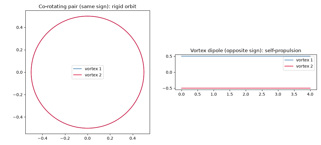
pair separation: started at 1.000, ended at 1.000 (conserved by rigid rotation)
dipole separation: started at 1.000, ended at 1.000 (conserved by rigid translation)