A von Karman vortex street holds its shape

Concentrating a 2D flow’s vorticity into point vortices turns the vorticity-transport PDE into an N-body system: each vortex simply advects with the velocity induced by every other vortex through the 2D Biot-Savart law,

\[\mathbf{u}(\mathbf{r}_i) = \sum_{j\neq i} \frac{\Gamma_j}{2\pi r_{ij}^2}\,\hat{\mathbf{z}}\times(\mathbf{r}_i-\mathbf{r}_j),\]

where \(\Gamma_j\) is vortex \(j\)’s circulation and \(r_{ij}=|\mathbf{r}_i-\mathbf{r}_j|\). Theodore von Karman showed that a staggered double row of point vortices – all clockwise in one row, all counterclockwise in the other – spaced by \(l\) along each row and separated across the rows by \(h\), is linearly stable to vortex-row perturbations at exactly one spacing ratio, VON_KARMAN_SPACING_RATIO (\(h/l \approx 0.2805\)) – the configuration nature seems to select behind every bluff body, from a chimney to a violin string in the wind. 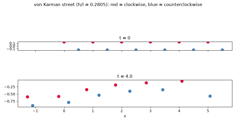This example builds that street with von_karman_vortex_street() and lets the full point-vortex N-body dynamics run: relative to the surrounding fluid, the staggered pattern should translate as a whole at \(U = \frac{\Gamma}{2l}\tanh(\pi h/l)\) (toward \(-x\), lagging the stream that shed it) without buckling.

import matplotlib.pyplot as plt
import numpy as np

from physicskit.fluids.systems.vortex_dynamics import PointVortexSystem, von_karman_vortex_street
from physicskit.fluids.visualizers import theme

Build the staggered street

positions0, circulations = von_karman_vortex_street(n_pairs=6, spacing_l=1.0)
street = PointVortexSystem(positions=positions0, circulations=circulations)

Advance the N-body dynamics

A finite street’s end vortices are not perfectly stabilized the way an infinite row would be (von Karman’s stability analysis assumes an infinite, perfectly periodic row), so the interior vortices are the ones that should hold their staggered spacing.

dt, n_steps = 0.01, 400
times, trajectory = street.trajectory(dt=dt, n_steps=n_steps)

Plot initial and final configurations

fig, axes = plt.subplots(2, 1, figsize=(9, 5), sharex=True)
colors = [theme.PRIMARY if c > 0 else theme.ACCENT for c in circulations]
axes[0].scatter(positions0[:, 0], positions0[:, 1], c=colors, s=60)
axes[0].set_title("t = 0")
axes[0].set_aspect("equal")

final = trajectory[-1]
axes[1].scatter(final[:, 0], final[:, 1], c=colors, s=60)
axes[1].set_title(f"t = {n_steps * dt:.1f}")
axes[1].set_aspect("equal")
axes[1].set_xlabel("x")
fig.suptitle("von Karman street (h/l = 0.2805): red = clockwise, blue = counterclockwise")
fig.tight_layout()

The full trajectories, not just two snapshots

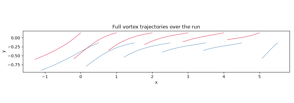
trajectory above already holds every vortex’s full path, not just its endpoints. Plotting all of it at once, rather than only the initial and final configurations, shows the staggered street translating as a whole – each vortex tracing a wavy but unbroken path – which is exactly what “holds its shape” means for a finite street’s interior.

fig, ax = plt.subplots(figsize=(10, 3.5))
for i in range(positions0.shape[0]):
    color = theme.PRIMARY if circulations[i] > 0 else theme.ACCENT
    ax.plot(trajectory[:, i, 0], trajectory[:, i, 1], color=color, lw=1.0, alpha=0.8)
ax.set_aspect("equal")
ax.set_xlabel("x")
ax.set_ylabel("y")
ax.set_title("Full vortex trajectories over the run")
fig.tight_layout()

interior = slice(2, -2)  # exclude the end vortices, which feel a finite-street edge effect
h_over_l_initial = np.std(positions0[interior, 1]) / 1.0
h_over_l_final = np.std(final[interior, 1]) / 1.0
print(f"interior row-spacing spread: t=0 -> {h_over_l_initial:.4f}, t={n_steps * dt:.1f} -> {h_over_l_final:.4f}")

plt.show()

interior row-spacing spread: t=0 -> 0.1403, t=4.0 -> 0.2063