Viscous decay under the Navier-Stokes equations

Navier (1822) and Stokes (1845) added a viscous friction term to Euler’s inviscid equations of motion, giving the equation that still governs essentially all of fluid dynamics today,

\[\partial_t\mathbf{u} + (\mathbf{u}\cdot\nabla)\mathbf{u} = -\nabla p/\rho + \nu\nabla^2\mathbf{u}.\]

NavierStokes2D solves the equivalent, pressure-free vorticity-transport form of exactly this equation in two dimensions, on a doubly periodic domain,

\[\partial_t \omega + (\mathbf{u}\cdot\nabla)\omega = \nu \nabla^2 \omega, \qquad \nabla^2\psi=-\omega, \qquad \mathbf{u}=(\partial_y\psi,\,-\partial_x\psi),\]

recovering the incompressible velocity \(\mathbf{u}\) from an exact spectral Poisson solve for the streamfunction \(\psi\) at every step. This example starts from a smooth, doubly periodic sinusoidal vortex patch \(\omega_0(x,y)=\sin x\sin y\) and shows the signature of the viscous term directly, as a steady decay of the patch’s peak vorticity.

import matplotlib.pyplot as plt
import numpy as np

from physicskit.fluids.systems.navier_stokes import NavierStokes2D
from physicskit.fluids.visualizers import theme
from physicskit.fluids.visualizers.flow_fields import plot_vorticity_field

A doubly periodic, sinusoidal vortex patch

n, length = 64, 2 * np.pi
solver = NavierStokes2D(n=n, length=length, nu=0.1)
omega0 = np.sin(solver.X) * np.sin(solver.Y)

Advance the vorticity-transport form of Navier-Stokes with RK4

Advancing in chunks (rather than one 200-step call) costs nothing extra – it is the same 200 RK4 steps in the same order – but lets the peak vorticity be recorded along the way, for the decay-rate check below.

dt, chunk, n_chunks = 0.01, 20, 10
omega = omega0.copy()
times, peaks = [0.0], [np.max(np.abs(omega0))]
for i in range(n_chunks):
    result = solver.simulate(omega, dt=dt, steps=chunk)
    omega = result["omega"]
    times.append((i + 1) * dt * chunk)
    peaks.append(np.max(np.abs(omega)))
times, peaks = np.array(times), np.array(peaks)

Viscosity \(\nu\nabla^2\omega\) steadily bleeds enstrophy out of the flow – the hallmark of the added friction term.

fig, ax = plot_vorticity_field(solver.X, solver.Y, result["omega"], result["u"], result["v"])
ax.set_title("Viscous decay of a periodic vortex patch")
fig.tight_layout()

print(f"max|omega|: {np.max(np.abs(omega0)):.4f} -> {np.max(np.abs(result['omega'])):.4f}")

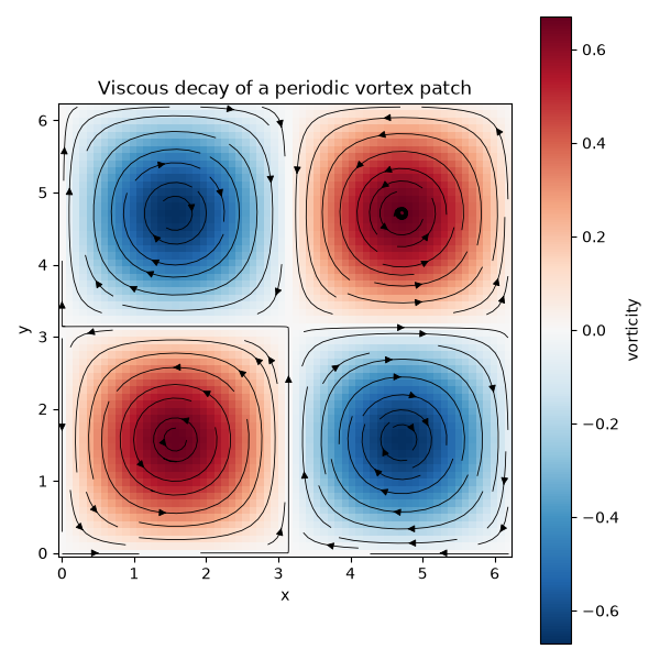
max|omega|: 1.0000 -> 0.6703

The decay rate itself, checked against pure diffusion

\(\omega_0=\sin x\sin y\) is an eigenmode of the Laplacian (\(\nabla^2\omega_0=-2\omega_0\)) whose induced streamfunction is exactly proportional to itself (\(\psi=\omega/2\) here), which makes the advecting velocity \((\partial_y\psi,-\partial_x\psi)\) everywhere perpendicular to \(\nabla\omega\) – so the nonlinear advection term \((\mathbf{u}\cdot\nabla)\omega\) vanishes identically and only viscous diffusion acts: the peak vorticity should decay as \(e^{-2\nu t}\), with no free parameters to fit.

analytic_decay = peaks[0] * np.exp(-2.0 * solver.nu * times)

fig, ax = plt.subplots(figsize=(6, 4))
ax.plot(times, peaks, "o", color=theme.PRIMARY, label="simulated max|omega|")
ax.plot(times, analytic_decay, color=theme.ACCENT, ls="--", label=r"$e^{-2\nu t}$ (pure diffusion)")
ax.set_xlabel("t")
ax.set_ylabel(r"max$|\omega|$")
ax.legend()
ax.set_title("Peak-vorticity decay matches pure diffusion exactly")
fig.tight_layout()

print(f"max relative deviation from e^(-2 nu t): {np.max(np.abs(peaks - analytic_decay) / analytic_decay):.2e}")

plt.show()

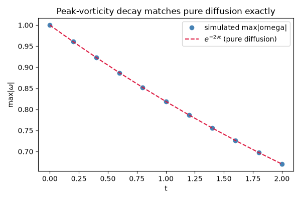
max relative deviation from e^(-2 nu t): 5.33e-14