The Blasius laminar boundary layer

Ludwig Prandtl’s 1904 boundary-layer theory reduced the full Navier-Stokes equations, in the thin-layer limit next to a wall, to a much simpler boundary-layer approximation; Paul Blasius then found, for steady, incompressible flow over a flat plate with zero streamwise pressure gradient, that the similarity substitution \(\eta = y\sqrt{U_\infty/(\nu x)}\), \(f(\eta)\) the dimensionless streamfunction, collapses even that approximation to a single third-order ordinary differential equation:

\[f''' + \tfrac{1}{2} f f'' = 0, \qquad f(0) = f'(0) = 0, \qquad f'(\infty) = 1,\]

with the streamwise velocity recovered as \(u/U_\infty = f'(\eta)\). The no-slip, no-penetration wall condition fixes \(f(0)=f'(0)=0\); the free-stream condition \(f'(\infty)=1\) is what makes this a two-point boundary value problem rather than an ordinary initial-value one. blasius_solve() solves it by shooting on the free parameter \(f''(0)\), and this example uses that solution to build the velocity profile, boundary-layer growth, and skin-friction scaling for a real flat-plate flow.

import matplotlib.pyplot as plt
import numpy as np

from physicskit.fluids.systems.viscous_flow import (
    blasius_boundary_layer_thickness,
    blasius_skin_friction_coefficient,
    blasius_solve,
)
from physicskit.fluids.visualizers import theme

The self-similar velocity profile

Every downstream station collapses onto the same curve \(u/U_\infty = f'(\eta)\) when plotted against the similarity variable \(\eta\).

result = blasius_solve()
print(f"Blasius wall-curvature constant f''(0) = {result['fpp'][0]:.5f} (classic value: 0.33206)")

fig, ax = plt.subplots(figsize=(5, 6))
ax.plot(result["fp"], result["eta"], color=theme.PRIMARY)
ax.set_xlabel(r"$u/U_\infty = f'(\eta)$")
ax.set_ylabel(r"$\eta$")
ax.invert_yaxis()
ax.set_title("Blasius similarity velocity profile")
fig.tight_layout()

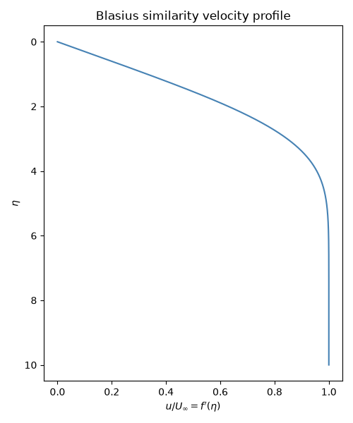
Blasius wall-curvature constant f''(0) = 0.33206 (classic value: 0.33206)

Boundary-layer growth and skin friction along a real plate

Converting back to physical units for air flowing over a 1-meter plate at a moderate speed shows both of the Blasius solution’s classic scalings: \(\delta_{99} \propto \sqrt{x}\) and \(c_f \propto Re_x^{-1/2}\).

U_inf, nu = 5.0, 1.5e-5  # air, m/s and m^2/s
x = np.linspace(0.01, 1.0, 200)
delta_99 = blasius_boundary_layer_thickness(x, U_inf, nu)
Re_x = U_inf * x / nu
cf = blasius_skin_friction_coefficient(Re_x, fpp0=result["fpp"][0])

fig, axes = plt.subplots(1, 2, figsize=(10, 4))
axes[0].plot(x, delta_99 * 1000, color=theme.PRIMARY)
axes[0].set_xlabel("x (m)")
axes[0].set_ylabel(r"$\delta_{99}$ (mm)")
axes[0].set_title("Boundary-layer thickness")

axes[1].loglog(Re_x, cf, color=theme.ACCENT)
axes[1].set_xlabel(r"$Re_x$")
axes[1].set_ylabel(r"$c_f$")
axes[1].set_title("Skin-friction coefficient")
fig.tight_layout()

print(f"boundary layer thickness at x=1m: {delta_99[-1] * 1000:.2f} mm (thin compared to the plate length)")

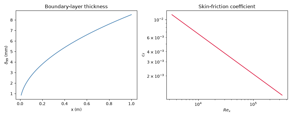
boundary layer thickness at x=1m: 8.50 mm (thin compared to the plate length)

The full 2D velocity field, not just one similarity profile

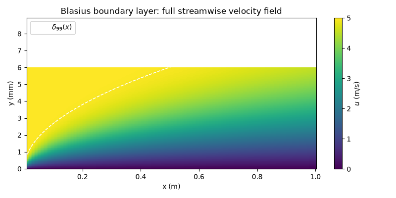
The similarity profile above is a single cross-section in the collapsed variable \(\eta\); substituting \(\eta=y\sqrt{U_\infty/(\nu x)}\) back in and reading \(f'(\eta)\) off the same blasius_solve() output at every physical \((x,y)\) rebuilds the full streamwise velocity field over the plate, showing directly how the boundary layer (bounded above by \(\delta_{99}(x)\)) thickens downstream while every vertical slice through it is secretly the same universal profile.

y_field = np.linspace(0.0, 6.0e-3, 150)  # m, above the delta_99 reached by x=1m
X_field, Y_field = np.meshgrid(x, y_field, indexing="ij")
eta_field = Y_field * np.sqrt(U_inf / (nu * X_field))
u_field = np.interp(eta_field, result["eta"], result["fp"]) * U_inf

fig, ax = plt.subplots(figsize=(8, 4))
im = ax.pcolormesh(X_field, Y_field * 1000, u_field, cmap=theme.SEQUENTIAL_CMAP, shading="auto")
fig.colorbar(im, ax=ax, label=r"$u$ (m/s)")
ax.plot(x, delta_99 * 1000, color="white", lw=1.2, ls="--", label=r"$\delta_{99}(x)$")
ax.set_xlabel("x (m)")
ax.set_ylabel("y (mm)")
ax.legend()
ax.set_title("Blasius boundary layer: full streamwise velocity field")
fig.tight_layout()

plt.show()