Couette versus Poiseuille flow

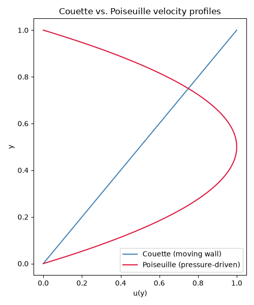
Both flows are steady, unidirectional shear flow between two infinite parallel plates separated by a gap \(h\), for which the full nonlinear Navier-Stokes equations collapse to a single linear ordinary differential equation for \(u(y)\):

\[\mu\,\frac{d^2u}{dy^2} = \frac{dp}{dx}.\]

The two classic problems differ only in what drives the flow and in the no-slip boundary conditions imposed at the walls \(y=0\) and \(y=h\). Plane Couette flow has no imposed pressure gradient (\(dp/dx=0\)) and drives the fluid purely by dragging the upper plate at speed \(U_{wall}\), i.e. \(u(0)=0\), \(u(h)=U_{wall}\), giving the straight-line profile \(u(y)=U_{wall}\,y/h\) of couette_flow_velocity(). Plane Poiseuille flow instead holds both plates at rest (\(u(0)=u(h)=0\)) and drives the fluid with a constant imposed pressure gradient \(dp/dx\), giving the parabolic profile \(u(y) = -\tfrac{1}{2\mu}\tfrac{dp}{dx}\,y\,(h-y)\) of poiseuille_flow_velocity(). Plotting them side by side on the same gap makes the contrast immediate.

import matplotlib.pyplot as plt
import numpy as np

from physicskit.fluids.systems.viscous_flow import (
    couette_flow_velocity,
    poiseuille_flow_rate,
    poiseuille_flow_velocity,
)
from physicskit.fluids.visualizers import theme

Two profiles on the same gap

The pressure gradient in the Poiseuille case is chosen so its peak velocity matches the Couette wall speed, isolating the shape difference.

h, U_wall, mu = 1.0, 1.0, 1.0
y = np.linspace(0, h, 200)

u_couette = couette_flow_velocity(y, U_wall=U_wall, h=h)
dpdx = -8.0 * mu * U_wall / h**2  # chosen so the Poiseuille peak also equals U_wall
u_poiseuille = poiseuille_flow_velocity(y, dpdx=dpdx, mu=mu, h=h)

fig, ax = plt.subplots(figsize=(5, 6))
ax.plot(u_couette, y, color=theme.PRIMARY, label="Couette (moving wall)")
ax.plot(u_poiseuille, y, color=theme.ACCENT, label="Poiseuille (pressure-driven)")
ax.set_xlabel("u(y)")
ax.set_ylabel("y")
ax.legend()
ax.set_title("Couette vs. Poiseuille velocity profiles")
fig.tight_layout()

The Poiseuille flow rate

Integrating the parabolic profile across the gap gives the volumetric flow rate per unit depth in closed form,

\[Q = -\frac{h^3}{12\mu}\frac{dp}{dx},\]

which poiseuille_flow_rate() returns directly, without needing to integrate the profile numerically.

Q = poiseuille_flow_rate(dpdx=dpdx, mu=mu, h=h)
print(f"Poiseuille volumetric flow rate per unit depth: Q = {Q:.4f}")

Poiseuille volumetric flow rate per unit depth: Q = 0.6667

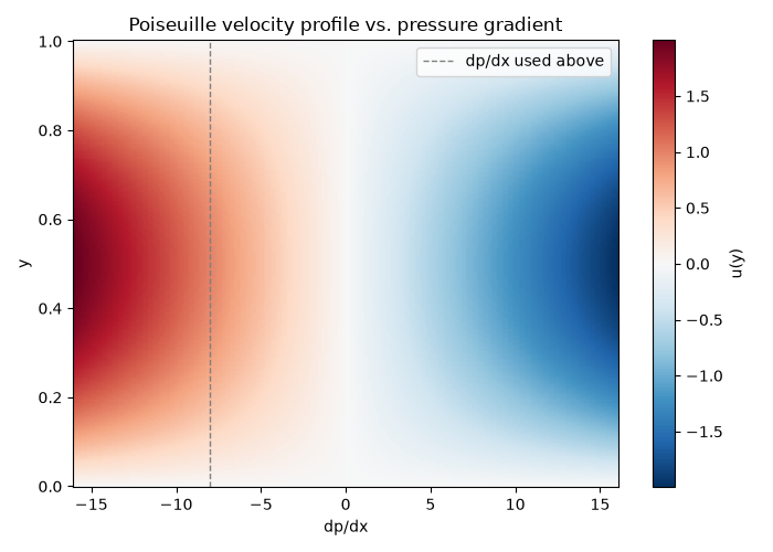
The Poiseuille profile across a full sweep of pressure gradients

The single profile above used one particular dpdx. Sweeping it turns the same closed-form poiseuille_flow_velocity() into a 2D map: reversing the pressure gradient’s sign reverses the flow direction while the no-slip walls keep every profile exactly parabolic in shape, and its magnitude alone sets the peak speed.

dpdx_sweep = np.linspace(-16.0, 16.0, 200)
Y_grid, DPDX_grid = np.meshgrid(y, dpdx_sweep, indexing="ij")
u_grid = poiseuille_flow_velocity(Y_grid, dpdx=DPDX_grid, mu=mu, h=h)
u_max = np.max(np.abs(u_grid))

fig, ax = plt.subplots(figsize=(7, 5))
im = ax.pcolormesh(dpdx_sweep, y, u_grid, cmap=theme.DIVERGING_CMAP, shading="auto", vmin=-u_max, vmax=u_max)
fig.colorbar(im, ax=ax, label="u(y)")
ax.axvline(dpdx, color=theme.MUTED, ls="--", lw=1.0, label="dp/dx used above")
ax.set_xlabel("dp/dx")
ax.set_ylabel("y")
ax.legend()
ax.set_title("Poiseuille velocity profile vs. pressure gradient")
fig.tight_layout()

plt.show()