Rayleigh-Bénard convection: the onset at a critical Rayleigh number

A fluid layer heated from below stays at rest, carrying heat by conduction, until the Rayleigh number

\[Ra = \frac{g\alpha\Delta T d^3}{\nu\kappa}\]

passes a critical value; then it overturns into convection rolls. Rayleigh (1916) found the threshold for stress-free walls, \(Ra_c = 27\pi^4/4 \approx 657.5\), and the rigid walls of Bénard’s experiments raise it to \(Ra_c \approx 1708\) at wavenumber \(a_c \approx 3.117\) (Jeffreys 1928; Pellew and Southwell 1940).

This example draws both marginal stability curves \(Ra(a)\), then integrates the nonlinear Boussinesq equations one critical wavelength wide, between stress-free walls and between rigid walls (Fourier in \(x\), Chebyshev in depth). Below onset a small perturbation decays; the growth rate crosses zero at 657.5 for stress-free walls and at 1708 for rigid ones. Above onset it grows into steady rolls whose heat flux exceeds conduction, \(Nu > 1\).

import matplotlib.pyplot as plt
import numpy as np

from physicskit.fluids.systems.convection import (
    RayleighBenard2D,
    RayleighBenardWalls2D,
    rayleigh_benard_critical,
    rayleigh_benard_growth_rate_free,
    rayleigh_benard_marginal_rayleigh,
)

Marginal stability curves for rigid and stress-free walls

Ra_rigid, a_rigid = rayleigh_benard_critical("rigid")
Ra_free, a_free = rayleigh_benard_critical("free")
a = np.linspace(1.0, 6.0, 80)
fig, axes = plt.subplots(1, 4, figsize=(17, 4))
axes[0].plot(a, [rayleigh_benard_marginal_rayleigh(ai, "rigid") for ai in a], color="navy", label="rigid (no-slip)")
axes[0].plot(a, [rayleigh_benard_marginal_rayleigh(ai, "free") for ai in a], color="darkorange", label="stress-free")
axes[0].plot([a_rigid], [Ra_rigid], "o", color="navy")
axes[0].plot([a_free], [Ra_free], "o", color="darkorange")
axes[0].annotate(f"$Ra_c = {Ra_rigid:.1f}$", (a_rigid, Ra_rigid), xytext=(a_rigid + 0.3, Ra_rigid - 450))
axes[0].annotate(f"$Ra_c = 27\\pi^4/4 = {Ra_free:.1f}$", (a_free, Ra_free), xytext=(a_free + 0.4, Ra_free - 300))
axes[0].set_ylim(0, 5000)
axes[0].set_xlabel("horizontal wavenumber a")
axes[0].set_ylabel("Ra")
axes[0].set_title("Convection above the curves")
axes[0].legend(loc="upper right")
print(f"rigid walls: Ra_c = {Ra_rigid:.2f} at a_c = {a_rigid:.3f}")
print(f"stress-free walls: Ra_c = {Ra_free:.2f} at a_c = {a_free:.3f}")

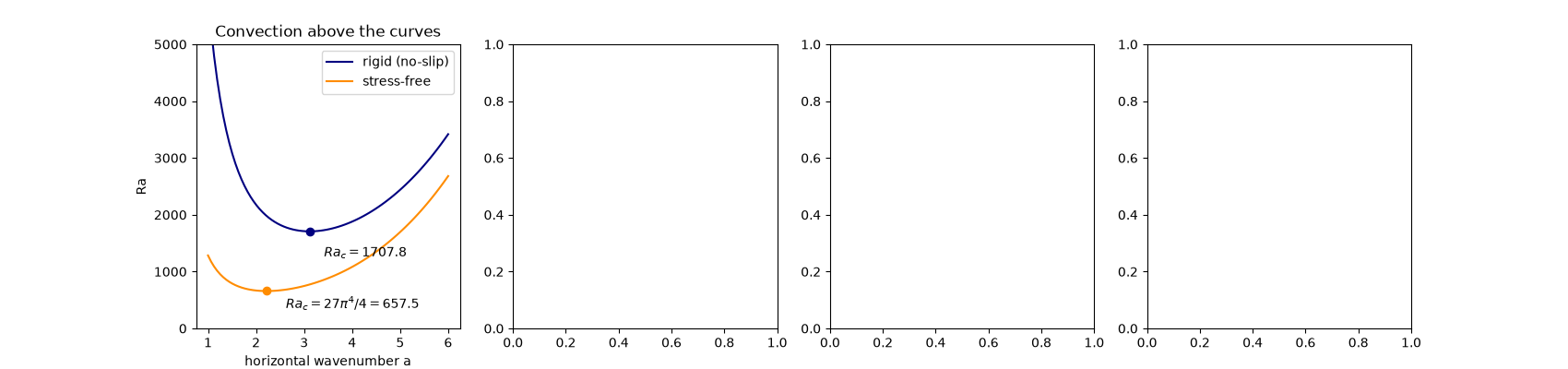
rigid walls: Ra_c = 1707.76 at a_c = 3.116
stress-free walls: Ra_c = 657.51 at a_c = 2.221

Linear growth rates from the nonlinear solvers

A small seeded roll grows or decays at a rate sigma(Ra) that crosses zero at the onset: the exact rate for stress-free walls, and the simulated rigid-wall rates crossing zero at Chandrasekhar’s 1708.

def growth_rate(rb, t_max, t_skip):
    rb.seed_mode(amplitude=1e-6)
    out = rb.run(t_max=t_max, dt=2e-3, sample_every=5)
    late = out["t"] > t_skip
    return np.polyfit(out["t"][late], np.log(np.abs(out["theta_mode"][late])), 1)[0]


Ra_scan = np.array([400.0, 550.0, 700.0, 900.0, 1200.0])
rates = np.array([growth_rate(RayleighBenard2D(Ra, nx=16, nz=16), 0.8, 0.3) for Ra in Ra_scan])
Ra_rigid_scan = np.array([1500.0, 1650.0, 1770.0, 1900.0, 2200.0])
rates_rigid = np.array([growth_rate(RayleighBenardWalls2D(Ra, nx=16, nz=20), 1.5, 0.5) for Ra in Ra_rigid_scan])
Ra_f = np.linspace(300, 1300, 200)
axes[1].plot(Ra_f, [rayleigh_benard_growth_rate_free(r, a_free) for r in Ra_f], "k-", label="stress-free, exact")
axes[1].plot(Ra_scan, rates, "o", color="darkorange", label="stress-free, simulated")
axes[1].plot(Ra_rigid_scan, rates_rigid, "s-", color="navy", label="rigid, simulated")
axes[1].axhline(0, color="gray", lw=0.5)
axes[1].axvline(Ra_free, color="darkorange", ls="--", lw=1)
axes[1].axvline(Ra_rigid, color="navy", ls="--", lw=1)
axes[1].set_xlabel("Ra")
axes[1].set_ylabel(r"growth rate $\sigma$ ($\kappa/d^2$)")
axes[1].set_title(r"Seeded roll at $a = a_c$, $Pr = 1$")
axes[1].legend(fontsize=7)
Ra_onset = np.interp(0.0, rates, Ra_scan)
Ra_onset_rigid = np.interp(0.0, rates_rigid, Ra_rigid_scan)

Nonlinear rolls and heat transport

Ra_values = np.array([600.0, 800.0, 1200.0, 2000.0, 3000.0])
Nu = []
for Ra in Ra_values:
    rb = RayleighBenard2D(Ra, nx=32, nz=32)
    rb.seed_mode(amplitude=1e-2)
    Nu.append(rb.run(t_max=6.0, dt=2e-3, sample_every=100)["nusselt"][-1])
    if Ra == 3000.0:
        rolls = rb
Nu = np.array(Nu)
axes[2].plot(Ra_values, Nu, "o-", color="crimson")
axes[2].axhline(1.0, color="gray", ls=":", label="conduction")
axes[2].axvline(Ra_free, color="darkorange", ls="--", lw=1)
axes[2].set_xlabel("Ra")
axes[2].set_ylabel("Nusselt number")
axes[2].set_title("Heat flux over conduction")
axes[2].legend()

half = rolls.z >= 0
_, w = rolls.velocity()
T = (1 - rolls.Z + rolls.theta)[half]
axes[3].contourf(rolls.x, rolls.z[half], T, levels=20, cmap="inferno")
u, _ = rolls.velocity()
axes[3].quiver(rolls.x[::2], rolls.z[half][::2], u[half][::2, ::2], w[half][::2, ::2], color="white")
axes[3].set_aspect("equal")
axes[3].set_xlabel("x / d")
axes[3].set_ylabel("z / d")
axes[3].set_title(f"Temperature and velocity, Ra = 3000, Nu = {Nu[-1]:.2f}")
plt.tight_layout()
plt.show()
print(f"simulated onset (sigma = 0): stress-free Ra = {Ra_onset:.1f}, rigid Ra = {Ra_onset_rigid:.1f}")
print(f"stress-free Nusselt numbers {np.round(Nu, 3)}")

simulated onset (sigma = 0): stress-free Ra = 659.3, rigid Ra = 1708.2
stress-free Nusselt numbers [1.    1.368 2.012 2.696 3.217]

Check

assert abs(Ra_rigid - 1707.76) < 0.05 and abs(a_rigid - 3.117) < 2e-3
np.testing.assert_allclose(rates, [rayleigh_benard_growth_rate_free(r, a_free) for r in Ra_scan], rtol=0.01, atol=0.01)
assert abs(Ra_onset - Ra_free) / Ra_free < 0.02
assert abs(Ra_onset_rigid - Ra_rigid) / Ra_rigid < 0.01
assert abs(Nu[0] - 1.0) < 1e-3 and np.all(Nu[1:] > 1.1)