Fourier’s heat equation: every mode decays on its own

Joseph Fourier’s Théorie analytique de la chaleur (1822) wrote heat conduction as

\[\frac{\partial u}{\partial t} = \alpha\,\nabla^2 u.\]

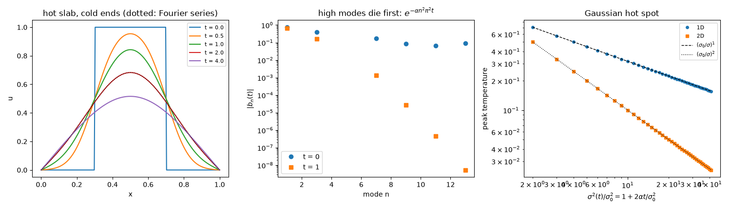
He solved it by expanding the initial temperature in sines and cosines. Each mode \(\sin kx\) decays on its own as \(e^{-\alpha k^2 t}\), so sharp features, which are made of high \(k\), vanish first. That expansion is the Fourier series.

This example follows a rod with a hot middle section and ice-cold ends, compares the Crank-Nicolson solution from heat_equation() with Fourier’s series, watches a Gaussian hot spot spread in 1D and 2D, and shows why the explicit scheme needs such small time steps.

import time

import matplotlib.pyplot as plt
import numpy as np

from physicskit.fluids import InvalidParameterError, gaussian_heat_solution, heat_equation, heat_equation_spectral

A hot slab between cold walls, mode by mode

A rod of length 1 is at \(u = 1\) for \(0.3 < x < 0.7\) and 0 elsewhere, with its ends held at 0. Fourier’s solution is \(u = \sum_n b_n \sin(n\pi x)\,e^{-\alpha n^2\pi^2 t}\). The two grid nodes sitting exactly on the jumps get the midpoint value 1/2, so the grid’s step is centered where the true one is.

alpha = 0.01
x = np.linspace(0.0, 1.0, 401)
u0 = np.where((x > 0.3) & (x < 0.7), 1.0, 0.0)
u0[np.isclose(x, 0.3) | np.isclose(x, 0.7)] = 0.5
times, frames = heat_equation(u0, x[1] - x[0], alpha, t_max=4.0, dt=0.005, n_frames=8)

n = np.arange(1, 400)
b_n = 2 / (n * np.pi) * (np.cos(0.3 * n * np.pi) - np.cos(0.7 * n * np.pi))


def fourier_series(t):
    return (b_n * np.exp(-alpha * (n * np.pi) ** 2 * t)) @ np.sin(np.outer(n, np.pi * x))


for t_k in (0.5, 4.0):
    k = np.argmin(np.abs(times - t_k))
    print(f"t = {times[k]:.2f}: max |Crank-Nicolson - Fourier series| = {np.max(np.abs(frames[k] - fourier_series(times[k]))):.1e}")

t = 0.50: max |Crank-Nicolson - Fourier series| = 1.5e-05
t = 4.00: max |Crank-Nicolson - Fourier series| = 2.2e-06

A Gaussian hot spot, in one and two dimensions

A Gaussian stays Gaussian with \(\sigma^2 = \sigma_0^2 + 2\alpha t\). Its peak falls as \((\sigma_0^2/\sigma^2)^{d/2}\): as \(t^{-1/2}\) on a line and \(t^{-1}\) on a plane, because the same heat spreads over more room.

g = np.linspace(-20, 20, 256, endpoint=False)
h = g[1] - g[0]
G1 = np.exp(-(g**2) / 2)
GX, GY = np.meshgrid(g, g, indexing="ij")
G2 = np.exp(-(GX**2 + GY**2) / 2)
t_g = np.linspace(0, 20, 41)
peak1 = heat_equation_spectral(G1, h, 1.0, t_g).max(axis=1)
peak2 = heat_equation_spectral(G2, h, 1.0, t_g).max(axis=(1, 2))

Explicit versus implicit time stepping

The explicit (FTCS) update is stable only for \(\alpha\Delta t/\Delta x^2 \le 1/2\), so halving \(\Delta x\) quarters the allowed step. Crank-Nicolson has no such limit.

dx = x[1] - x[0]
dt_max = 0.5 * dx**2 / alpha
try:
    heat_equation(u0, dx, alpha, t_max=1.0, dt=1.05 * dt_max, method="explicit")
except InvalidParameterError as err:
    print(f"explicit scheme refused: {err}")
t0 = time.perf_counter()
_, ex = heat_equation(u0, dx, alpha, t_max=1.0, dt=dt_max, method="explicit")
t_ex = time.perf_counter() - t0
t0 = time.perf_counter()
_, cn = heat_equation(u0, dx, alpha, t_max=1.0, dt=0.01)
t_cn = time.perf_counter() - t0
print(f"explicit: {round(1.0 / dt_max)} steps in {t_ex * 1e3:.0f} ms; Crank-Nicolson: 100 steps in {t_cn * 1e3:.0f} ms")
print(f"difference at t = 1: {np.max(np.abs(ex[-1] - cn[-1])):.1e}")

fig, axes = plt.subplots(1, 3, figsize=(15, 4.3))
for k in (0, 1, 2, 4, 8):
    axes[0].plot(x, frames[k], label=f"t = {times[k]:.1f}")
axes[0].plot(x, fourier_series(times[4]), "k:", lw=1)
axes[0].set_xlabel("x")
axes[0].set_ylabel("u")
axes[0].set_title("hot slab, cold ends (dotted: Fourier series)")
axes[0].legend(fontsize=8)

odd = n[:15][np.abs(b_n[:15]) > 1e-12]  # the even modes vanish by symmetry
axes[1].semilogy(odd, np.abs(b_n[odd - 1]), "o", label="t = 0")
axes[1].semilogy(odd, np.abs(b_n[odd - 1]) * np.exp(-alpha * (odd * np.pi) ** 2 * 1.0), "s", label="t = 1")
axes[1].set_xlabel("mode n")
axes[1].set_ylabel(r"$|b_n(t)|$")
axes[1].set_title(r"high modes die first: $e^{-\alpha n^2\pi^2 t}$")
axes[1].legend()

axes[2].loglog(1 + 2 * t_g[1:], peak1[1:], "o", ms=4, label="1D")
axes[2].loglog(1 + 2 * t_g[1:], peak2[1:], "s", ms=4, label="2D")
s2 = 1 + 2 * t_g[1:]
axes[2].loglog(s2, s2**-0.5, "k--", lw=1, label=r"$(\sigma_0/\sigma)^{1}$")
axes[2].loglog(s2, s2**-1.0, "k:", lw=1, label=r"$(\sigma_0/\sigma)^{2}$")
axes[2].set_xlabel(r"$\sigma^2(t)/\sigma_0^2 = 1 + 2\alpha t/\sigma_0^2$")
axes[2].set_ylabel("peak temperature")
axes[2].set_title("Gaussian hot spot")
axes[2].legend(fontsize=8)
fig.tight_layout()
print(f"1D peak at t = 20: {peak1[-1]:.4f}, closed form {gaussian_heat_solution(np.array([0.0]), 20.0, 1.0, 1.0)[0]:.4f}")
plt.show()

explicit scheme refused: explicit scheme unstable: alpha*dt*sum(1/dx^2) = 0.525 > 1/2; reduce dt or use crank_nicolson
explicit: 3200 steps in 6 ms; Crank-Nicolson: 100 steps in 2 ms
difference at t = 1: 4.9e-05
1D peak at t = 20: 0.1562, closed form 0.1562

Check

Crank-Nicolson reproduces the Fourier-series solution; the explicit scheme refuses dt above dx^2 / 2 alpha; a Gaussian hot spot’s peak falls as (sigma0 / sigma)^d with sigma^2 = sigma0^2 + 2 alpha t.

for t_k in (0.5, 4.0):
    k = np.argmin(np.abs(times - t_k))
    assert np.max(np.abs(frames[k] - fourier_series(times[k]))) < 1e-4
assert np.max(np.abs(ex[-1] - cn[-1])) < 1e-3
np.testing.assert_allclose(peak1, (1 + 2 * t_g) ** -0.5, rtol=1e-6)
np.testing.assert_allclose(peak2, (1 + 2 * t_g) ** -1.0, rtol=1e-6)