Chadwick’s neutron and the Weizsacker semi-empirical mass formula

Chadwick (1932) replaced the proton-electron nucleus with the modern picture: a nucleus of mass number \(A\) and atomic number \(Z\) is exactly \(Z\) protons and \(N=A-Z\) neutrons. Three years later, Weizsacker combined this proton-neutron picture with a liquid-drop model into a single closed-form estimate of nuclear binding energy,

\[B(Z,A) = a_V A - a_S A^{2/3} - a_C\frac{Z(Z-1)}{A^{1/3}} - a_A\frac{(A-2Z)^2}{A} + \delta(A,Z),\]

that presupposes exactly Chadwick’s \(N=A-Z\) bookkeeping – it has no way to vary the neutron number independently of \(Z\) in the proton-electron model it replaced. This example plots semf_binding_energy() across the \((N, Z)\) plane, and shows the asymmetry term’s role directly: for fixed \(A\), binding energy peaks not at \(Z=A/2\) but at the \(Z\) a real “valley of stability” nuclide actually sits at, because Coulomb repulsion among protons pulls the optimum below \(N=Z\).

import matplotlib.pyplot as plt
import numpy as np

from physicskit.particle.nuclear import binding_energy_per_nucleon, semf_binding_energy

The (N, Z) plane: binding energy and the valley of stability

For each mass number A, the most stable Z is the one maximizing B(Z,A) – fixing a “valley” of maximum binding energy that the semf alone, via its competing Coulomb and asymmetry terms, predicts without any experimental input.

A_values = np.arange(10, 220, 2)
Z_optimal = []
for A in A_values:
    Z_range = np.arange(1, A)
    B_values = np.array([semf_binding_energy(Z, A) for Z in Z_range])
    Z_optimal.append(Z_range[np.argmax(B_values)])
Z_optimal = np.array(Z_optimal)

fig1, ax1 = plt.subplots(figsize=(6.5, 5))
ax1.plot(A_values, Z_optimal, color="steelblue", label="Z maximizing B(Z,A) (SEMF valley of stability)")
ax1.plot(A_values, A_values / 2.0, "--", color="0.6", label="N=Z line")
ax1.set_xlabel("mass number A")
ax1.set_ylabel("Z")
ax1.set_title("The valley of stability: Coulomb repulsion favors N > Z for heavy nuclei")
ax1.legend(fontsize=8)
fig1.tight_layout()

print(f"at A=20:  most stable Z (SEMF) = {Z_optimal[np.argmin(np.abs(A_values - 20))]} (N=Z line would say 10)")
print(f"at A=120: most stable Z (SEMF) = {Z_optimal[np.argmin(np.abs(A_values - 120))]} (N=Z line would say 60)")
print(f"at A=200: most stable Z (SEMF) = {Z_optimal[np.argmin(np.abs(A_values - 200))]} (N=Z line would say 100)")
print("(heavier nuclei need progressively more neutrons than protons -- exactly the observed valley of stability)")

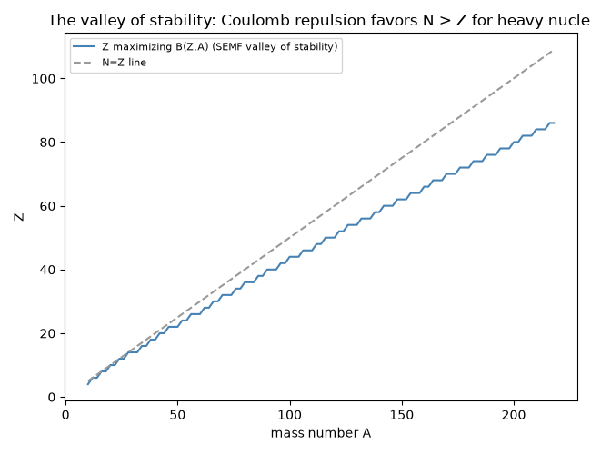
at A=20:  most stable Z (SEMF) = 10 (N=Z line would say 10)
at A=120: most stable Z (SEMF) = 50 (N=Z line would say 60)
at A=200: most stable Z (SEMF) = 80 (N=Z line would say 100)
(heavier nuclei need progressively more neutrons than protons -- exactly the observed valley of stability)

Fixing A: why the optimum is not at Z=A/2

For a single, concrete mass number, plotting binding energy directly against Z shows why: the asymmetry term alone would peak exactly at Z=A/2, but Coulomb repulsion (which grows with Z^2) tilts the peak toward smaller Z as A grows.

A_fixed = 120
Z_range = np.arange(1, A_fixed)
B_fixed = np.array([semf_binding_energy(Z, A_fixed) for Z in Z_range]) / A_fixed  # per nucleon

fig2, ax2 = plt.subplots(figsize=(6, 4.5))
ax2.plot(Z_range, B_fixed, color="firebrick")
ax2.axvline(A_fixed / 2, color="0.6", ls="--", label="Z=A/2 (no Coulomb term would peak here)")
i_max = np.argmax(B_fixed)
ax2.axvline(Z_range[i_max], color="steelblue", ls="--", label=f"actual peak, Z={Z_range[i_max]}")
ax2.set_xlabel("Z (at fixed A=120)")
ax2.set_ylabel("binding energy per nucleon (MeV)")
ax2.set_title("Coulomb repulsion shifts the optimal Z below A/2")
ax2.legend(fontsize=8)
fig2.tight_layout()

print(f"\nat A={A_fixed}: binding-energy-per-nucleon peaks at Z={Z_range[i_max]} (N-Z={A_fixed - 2 * Z_range[i_max]}), not at Z=A/2={A_fixed / 2}")

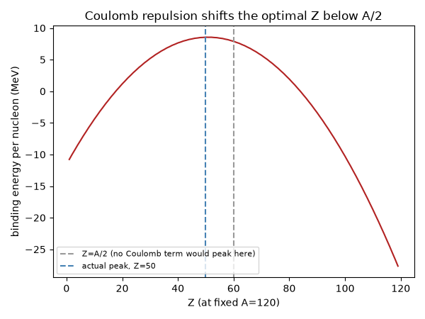
at A=120: binding-energy-per-nucleon peaks at Z=50 (N-Z=20), not at Z=A/2=60.0

The pairing term: even-even nuclei are slightly more bound

Chadwick’s proton-neutron picture also makes the small pairing correction meaningful (it depends on the parity of both Z and N separately) – something with no analogue in a proton-electron model.

for Z, A, label in [(50, 120, "even-even (Z=50,N=70)"), (51, 120, "odd-odd (Z=51,N=69)")]:
    bpn = binding_energy_per_nucleon(Z, A)
    print(f"{label}: binding energy/nucleon = {bpn:.4f} MeV")

plt.show()

even-even (Z=50,N=70): binding energy/nucleon = 8.5484 MeV
odd-odd (Z=51,N=69): binding energy/nucleon = 8.5363 MeV