Dispersion, twin-slit interference, and quantum revivals

Three non-stationary phenomena governed by the time-dependent Schrodinger equation, each solved via its own exact analytic route rather than direct numerical propagation. A free Gaussian wavepacket keeps its Gaussian shape but spreads as it travels, its width growing as

\[\sigma(t) = \sigma_0\sqrt{1 + \left(\frac{\hbar t}{2m\sigma_0^2}\right)^2}.\]

A matter-wave analogue of Young’s experiment sends the same kind of packet through two coherent point sources (slits) separated by a fixed distance; the two paraxially-propagated contributions interfere on a downstream screen, building up the intensity \(\lvert\psi_1+\psi_2\rvert^2\). Finally, a wavepacket confined to an infinite square well of width \(L\) – whose eigenenergies \(E_n=n^2\pi^2\hbar^2/(2mL^2)\) grow quadratically in \(n\) – disperses into an apparently chaotic superposition yet exactly reassembles into a replica of its initial shape at the revival time \(t_\text{rev}=4mL^2/(\pi\hbar)\) (with a mirror-image replica at \(t_\text{rev}/2\)), a purely quantum consequence of the discrete, quadratically-spaced spectrum.

import matplotlib.pyplot as plt
import numpy as np

from physicskit.quantum.chapters.wave_packets import GaussianDispersion, QuantumRevival, TwinSlit
from physicskit.quantum.visualizers.wavefunctions import animate_density

Free dispersion, twin-slit interference, and quantum revivals

fig, axes = plt.subplots(1, 3, figsize=(15, 4.5))

# Free-particle dispersion: width grows, exact analytic solution
gd = GaussianDispersion(x0=0.0, sigma0=1.0, k0=3.0)
x1 = np.linspace(-20, 40, 1000)
for t in [0, 2, 5, 10]:
    axes[0].plot(x1, gd.density(x1, t), label=f"t={t}")
axes[0].set_title("Free wavepacket dispersion\n(width grows, exact analytic solution)")
axes[0].set_xlabel("x")
axes[0].legend(fontsize=8)

# Twin-slit interference: the matter-wave analogue of Young's experiment
ts = TwinSlit(slit_separation=4.0, slit_width=0.4, k0=10.0)
x2 = np.linspace(-10, 10, 2000)
I = ts.intensity(x2, screen_distance=50)
axes[1].plot(x2, I)
axes[1].set_title("Twin-slit interference\n(matter-wave analogue of Young's experiment)")
axes[1].set_xlabel("screen position")

# Quantum revivals in the infinite square well: dispersion -> exact self-reassembly
qr = QuantumRevival(L=1.0, n_max=300)
x3 = np.linspace(0, qr.L, 1500)
psi0_func = qr.gaussian_initial_state(x0=0.3, sigma=0.03)
psi0 = psi0_func(x3)
coeffs = qr.eigenbasis_coefficients(psi0_func)

t_rev = qr.revival_time
fractions = [0.0, 0.25, 0.5, 1.0]
offset = 0
for frac in fractions:
    density = np.abs(qr.wavefunction(x3, frac * t_rev, coeffs)) ** 2
    axes[2].plot(x3, density + offset, label=f"t={frac:.2f} t_rev")
    offset += density.max() * 1.3
# infinite walls of the box, for reference
axes[2].axvline(0.0, color="black", lw=1.2)
axes[2].axvline(qr.L, color="black", lw=1.2)
axes[2].set_title("Quantum revivals in an infinite well [0,L]\n(dispersion -> exact self-reassembly)")
axes[2].set_xlabel("x")
axes[2].legend(fontsize=7)

fig.tight_layout()

Fidelity to the initial state approaches 1 at (fractional) revival times.

for frac in fractions:
    fid = qr.fidelity_to_initial(x3, frac * t_rev, coeffs, psi0)
    print(f"fidelity to initial state at t={frac} t_rev: {fid:.4f}")

fidelity to initial state at t=0.0 t_rev: 1.0000
fidelity to initial state at t=0.25 t_rev: 0.5000
fidelity to initial state at t=0.5 t_rev: 0.0000
fidelity to initial state at t=1.0 t_rev: 1.0000

An animated view of free dispersion

The static snapshots of gd.density above come from trajectory(), the same exact analytic free-particle solution stacked over a time grid, shaped for animate_density() – here rendered phase-colored, so the de Broglie phase \(e^{ik_0x}\) riding along the ballistically advancing center is directly visible while the envelope spreads.

t_anim = np.linspace(0, 6.0, 120)
x_anim = np.linspace(-20, 40, 600)
frames = gd.trajectory(x_anim, t_anim)
anim = animate_density(x_anim, frames, times=t_anim)
# anim.save("wave_packet_dispersion.gif", writer="pillow", fps=15)

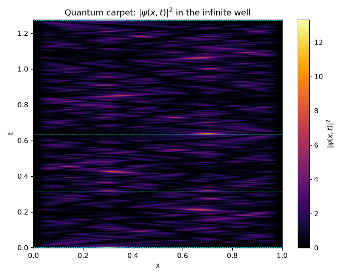
A “quantum carpet”: the full space-time revival pattern

The four discrete snapshots above sample wavefunction() at isolated fractions of \(t_\text{rev}\); evaluating it on a full \((x,t)\) grid instead reveals the famous “quantum carpet” – a web of diagonal fractional-revival ridges that the discrete snapshots only hint at, converging back to sharp replicas of the initial state exactly at \(t=0\), \(t_\text{rev}/2\), and \(t_\text{rev}\).

t_carpet = np.linspace(0, t_rev, 500)
x_carpet = np.linspace(0, qr.L, 700)
carpet = np.array([np.abs(qr.wavefunction(x_carpet, t, coeffs)) ** 2 for t in t_carpet])

fig2, ax4 = plt.subplots(figsize=(7, 5.5))
im = ax4.pcolormesh(x_carpet, t_carpet, carpet, shading="auto", cmap="inferno")
for frac in fractions:
    ax4.axhline(frac * t_rev, color="cyan", ls="--", lw=0.6)
ax4.set_xlabel("x")
ax4.set_ylabel("t")
ax4.set_title(r"Quantum carpet: $|\psi(x,t)|^2$ in the infinite well")
fig2.colorbar(im, ax=ax4, label=r"$|\psi(x,t)|^2$")
fig2.tight_layout()