Legendre and Gauss’s least squares: fitting a calibration line

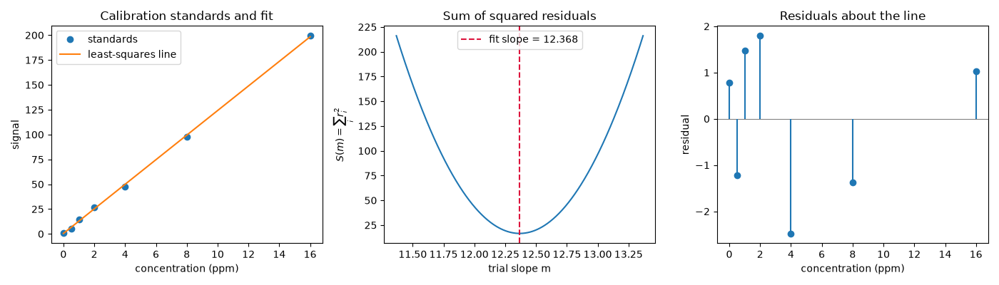
The method of least squares picks the straight line that minimizes the sum of squared residuals \(S(m,b)=\sum_i(y_i-mx_i-b)^2\). fit_calibration() performs exactly that fit for a set of calibration standards; here we check that its slope sits at the bottom of the \(S(m)\) parabola, and that the residuals it leaves behind scatter around zero.

import matplotlib.pyplot as plt
import numpy as np

from chemistrykit.analytical import fit_calibration

rng = np.random.default_rng(42)
concentration = np.array([0.0, 0.5, 1.0, 2.0, 4.0, 8.0, 16.0])  # ppm
true_slope, true_intercept, noise_sigma = 12.4, 0.8, 1.5
signal = true_slope * concentration + true_intercept + rng.normal(scale=noise_sigma, size=concentration.shape)

cal = fit_calibration(concentration, signal)
print(f"Least-squares slope:     {cal.slope:.4f} (true {true_slope})")
print(f"Least-squares intercept: {cal.intercept:.4f} (true {true_intercept})")
print(f"R^2 = {cal.r_squared:.6f}")

Least-squares slope:     12.3677 (true 12.4)
Least-squares intercept: 0.4806 (true 0.8)
R^2 = 0.999456

The sum of squared residuals as a function of trial slope (with the intercept re-optimized for each slope) is a parabola whose minimum is the least-squares slope – Legendre’s criterion made visible:

trial_slopes = np.linspace(cal.slope - 1.0, cal.slope + 1.0, 401)
x_mean, y_mean = concentration.mean(), signal.mean()
S = np.array([np.sum((signal - (m * concentration + (y_mean - m * x_mean))) ** 2) for m in trial_slopes])
print(f"\nSlope minimizing S on the scan: {trial_slopes[np.argmin(S)]:.4f}")

residuals = signal - cal.predict_signal(concentration)
print(f"Sum of residuals (zero for a least-squares line with intercept): {residuals.sum():.2e}")

Slope minimizing S on the scan: 12.3677
Sum of residuals (zero for a least-squares line with intercept): -1.99e-13

fig, axes = plt.subplots(1, 3, figsize=(14, 4))
c_line = np.linspace(0, concentration.max(), 100)
axes[0].plot(concentration, signal, "o", label="standards")
axes[0].plot(c_line, cal.predict_signal(c_line), "-", label="least-squares line")
axes[0].set_xlabel("concentration (ppm)")
axes[0].set_ylabel("signal")
axes[0].set_title("Calibration standards and fit")
axes[0].legend()

axes[1].plot(trial_slopes, S)
axes[1].axvline(cal.slope, color="crimson", linestyle="--", label=f"fit slope = {cal.slope:.3f}")
axes[1].set_xlabel("trial slope m")
axes[1].set_ylabel(r"$S(m)=\sum_i r_i^2$")
axes[1].set_title("Sum of squared residuals")
axes[1].legend()

axes[2].axhline(0.0, color="gray", linewidth=0.8)
axes[2].vlines(concentration, 0.0, residuals, color="C0")
axes[2].plot(concentration, residuals, "o")
axes[2].set_xlabel("concentration (ppm)")
axes[2].set_ylabel("residual")
axes[2].set_title("Residuals about the line")
plt.tight_layout()
plt.show()