Limits of detection and quantitation from a calibration curve

Long and Winefordner argued that a detection limit should be tied to the calibration’s own residual scatter \(s_{y/x}\) and slope m. lod() and loq() use the widely adopted calibration-based convention \(\text{LOD}=3.3\,s_{y/x}/m\) and \(\text{LOQ}=10\,s_{y/x}/m\). A noisier method has proportionally higher limits.

import matplotlib.pyplot as plt
import numpy as np

from chemistrykit.analytical import fit_calibration
from chemistrykit.analytical.visualizers.analytical_plots import plot_calibration_curve

rng = np.random.default_rng(7)
concentration = np.array([0.0, 0.5, 1.0, 2.0, 4.0, 8.0, 16.0])  # ppm
slope, intercept = 12.4, 0.8

calibrations = {}
for noise in (1.5, 6.0):
    signal = slope * concentration + intercept + rng.normal(scale=noise, size=concentration.shape)
    cal = fit_calibration(concentration, signal)
    calibrations[noise] = (signal, cal)
    print(f"noise sigma={noise}: s_y/x={cal.residual_std_error:.3f}, LOD={cal.lod():.3f} ppm, LOQ={cal.loq():.3f} ppm, LOQ/LOD={cal.loq() / cal.lod():.4f}")

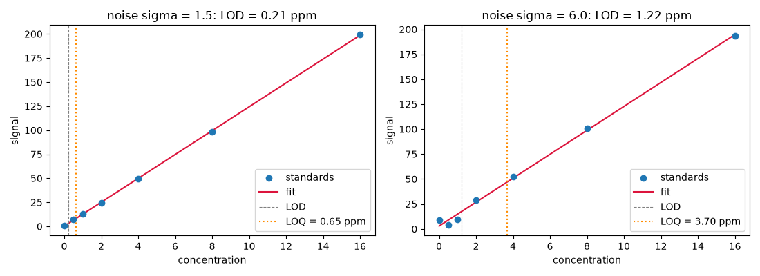
noise sigma=1.5: s_y/x=0.801, LOD=0.213 ppm, LOQ=0.646 ppm, LOQ/LOD=3.0303
noise sigma=6.0: s_y/x=4.432, LOD=1.220 ppm, LOQ=3.696 ppm, LOQ/LOD=3.0303

The signal levels corresponding to the two limits sit 3.3 and 10 residual standard deviations above the fitted blank (the intercept):

signal_lo, cal_lo = calibrations[1.5]
print(f"\nBlank (intercept): {cal_lo.intercept:.3f}")
print(f"Signal at LOD: {cal_lo.predict_signal(cal_lo.lod()):.3f} = blank + 3.3 s_y/x")
print(f"Signal at LOQ: {cal_lo.predict_signal(cal_lo.loq()):.3f} = blank + 10 s_y/x")

Blank (intercept): 0.337
Signal at LOD: 2.980 = blank + 3.3 s_y/x
Signal at LOQ: 8.347 = blank + 10 s_y/x

fig, axes = plt.subplots(1, 2, figsize=(11, 4))
for ax, (noise, (signal, cal)) in zip(axes, calibrations.items()):
    plot_calibration_curve(concentration, signal, calibration=cal, lod=cal.lod(), ax=ax)
    ax.axvline(cal.loq(), color="darkorange", linestyle=":", label=f"LOQ = {cal.loq():.2f} ppm")
    ax.set_title(f"noise sigma = {noise}: LOD = {cal.lod():.2f} ppm")
    ax.legend()
plt.tight_layout()
plt.show()