The van Deemter equation and the optimum flow velocity

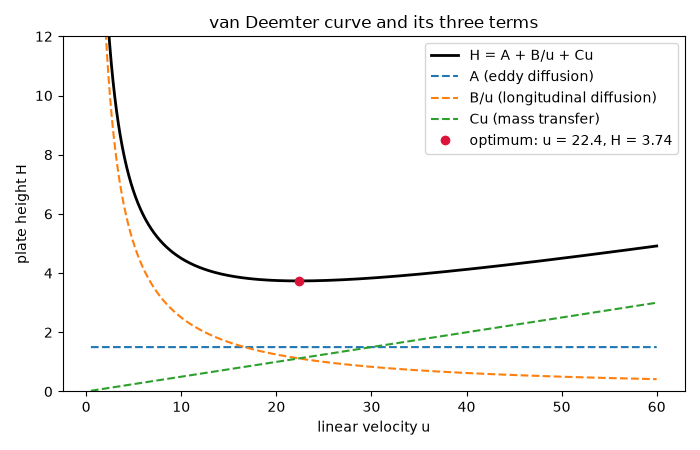
van_deemter_H() evaluates \(H=A+B/u+Cu\), the sum of eddy diffusion (A), longitudinal diffusion (B/u, dominant at low flow) and mass-transfer resistance (Cu, dominant at high flow). The competition between the last two gives a minimum plate height \(H_{min}=A+2\sqrt{BC}\) at \(u_{opt}=\sqrt{B/C}\) (minimum_plate_height(), optimum_flow_velocity()).

import matplotlib.pyplot as plt
import numpy as np

from chemistrykit.analytical import minimum_plate_height, optimum_flow_velocity, van_deemter_H

A, B, C = 1.5, 25.0, 0.05  # plate height in units of 1e-3 cm, u in cm/s
u = np.linspace(0.5, 60.0, 3000)
H = van_deemter_H(u, A, B, C)
u_opt = optimum_flow_velocity(B, C)
H_min = minimum_plate_height(A, B, C)
print(f"u_opt = sqrt(B/C) = {u_opt:.3f}; numerical minimum at u = {u[np.argmin(H)]:.3f}")
print(f"H_min = A + 2 sqrt(BC) = {H_min:.4f}; numerical minimum H = {H.min():.4f}")
print(f"At u_opt the B and C terms are equal: B/u = {B / u_opt:.4f}, Cu = {C * u_opt:.4f}")

u_opt = sqrt(B/C) = 22.361; numerical minimum at u = 22.364
H_min = A + 2 sqrt(BC) = 3.7361; numerical minimum H = 3.7361
At u_opt the B and C terms are equal: B/u = 1.1180, Cu = 1.1180

fig, ax = plt.subplots(figsize=(7, 4.5))
ax.plot(u, H, color="black", linewidth=2, label="H = A + B/u + Cu")
ax.plot(u, np.full_like(u, A), "--", label="A (eddy diffusion)")
ax.plot(u, B / u, "--", label="B/u (longitudinal diffusion)")
ax.plot(u, C * u, "--", label="Cu (mass transfer)")
ax.plot([u_opt], [H_min], "o", color="crimson", label=f"optimum: u = {u_opt:.1f}, H = {H_min:.2f}")
ax.set_ylim(0, 12)
ax.set_xlabel("linear velocity u")
ax.set_ylabel("plate height H")
ax.set_title("van Deemter curve and its three terms")
ax.legend()
plt.tight_layout()
plt.show()