Martin and Synge’s theoretical plates from a peak’s width

Treating a column as N equilibration stages (“theoretical plates”) predicts a Gaussian peak whose width grows as \(t_R/\sqrt N\). theoretical_plates() inverts that: \(N=16(t_R/w_{base})^2=5.545(t_R/w_{1/2})^2\), and plate_height() gives the plate height \(H=L/N\). Here we measure the widths of simulated peaks and recover the plate count they were built from.

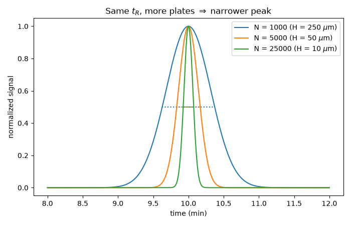
N built in =    1000: from FWHM 0.7444 min -> N =    1001; from base width -> N =    1000; H = 249.8 um
N built in =    5000: from FWHM 0.3328 min -> N =    5007; from base width -> N =    5000; H = 49.9 um
N built in =   25000: from FWHM 0.1488 min -> N =   25044; from base width -> N =   25000; H = 10.0 um

import matplotlib.pyplot as plt
import numpy as np

from chemistrykit.analytical import plate_height, simulate_chromatogram, theoretical_plates

t = np.linspace(8.0, 12.0, 20001)
column_length = 25.0  # cm
fig, ax = plt.subplots(figsize=(7, 4.5))
for N_true in (1000.0, 5000.0, 25000.0):
    peak = simulate_chromatogram(t, centers=[10.0], N=N_true)
    above = t[peak >= peak.max() / 2]
    w_half = above.max() - above.min()
    sigma = 10.0 / np.sqrt(N_true)
    N_half = theoretical_plates(10.0, w_half, width_type="half_height")
    N_base = theoretical_plates(10.0, 4.0 * sigma, width_type="base")
    H = plate_height(column_length, N_half)
    print(f"N built in = {N_true:7.0f}: from FWHM {w_half:.4f} min -> N = {N_half:7.0f}; from base width -> N = {N_base:7.0f}; H = {H * 1e4:.1f} um")
    ax.plot(t, peak / peak.max(), label=f"N = {N_true:.0f} (H = {H * 1e4:.0f} $\\mu$m)")
    ax.hlines(0.5, 10.0 - w_half / 2, 10.0 + w_half / 2, color=ax.lines[-1].get_color(), linestyle=":")

ax.set_xlabel("time (min)")
ax.set_ylabel("normalized signal")
ax.set_title(r"Same $t_R$, more plates $\Rightarrow$ narrower peak")
ax.legend()
plt.tight_layout()
plt.show()