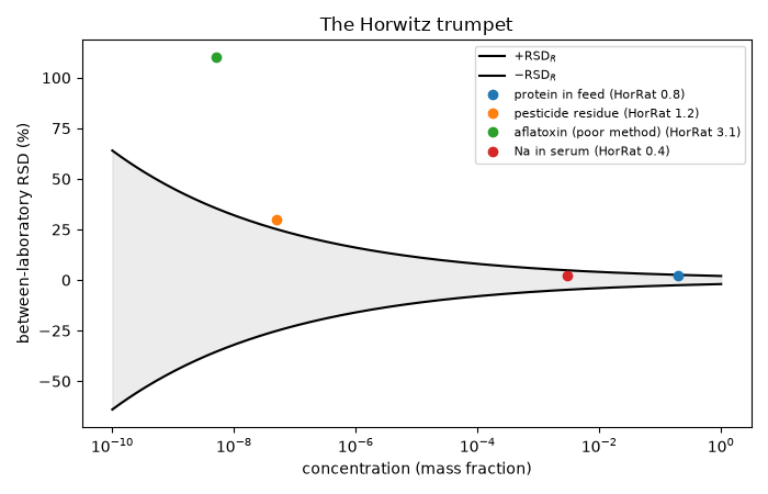
The Horwitz trumpet: interlaboratory precision vs. concentration

horwitz_rsd() gives Horwitz’s empirical expected between-laboratory RSD, \(2^{1-0.5\log_{10}C}\), which doubles for every 100-fold drop in concentration. Plotted as \(\pm\text{RSD}\) against concentration it opens like a trumpet. horrat() scores a method’s observed RSD against it.

import matplotlib.pyplot as plt
import numpy as np

from chemistrykit.analytical import horrat, horwitz_rsd

for label, C in [("pure substance", 1.0), ("1 %", 1e-2), ("1 ppm", 1e-6), ("1 ppb", 1e-9)]:
    print(f"{label:15s}: predicted RSD_R = {horwitz_rsd(C):5.1f} %")

pure substance : predicted RSD_R =   2.0 %
1 %            : predicted RSD_R =   4.0 %
1 ppm          : predicted RSD_R =  16.0 %
1 ppb          : predicted RSD_R =  45.3 %

Hypothetical collaborative-study results: (mass fraction, observed RSD %)

studies = {"protein in feed": (0.2, 2.1), "pesticide residue": (5e-8, 30.0), "aflatoxin (poor method)": (5e-9, 110.0), "Na in serum": (3e-3, 2.0)}
print()
for name, (C, rsd) in studies.items():
    print(f"{name:24s}: observed {rsd:5.1f} %, Horwitz {horwitz_rsd(C):5.1f} %, HorRat = {horrat(rsd, C):.2f}")

protein in feed         : observed   2.1 %, Horwitz   2.5 %, HorRat = 0.82
pesticide residue       : observed  30.0 %, Horwitz  25.1 %, HorRat = 1.19
aflatoxin (poor method) : observed 110.0 %, Horwitz  35.5 %, HorRat = 3.10
Na in serum             : observed   2.0 %, Horwitz   4.8 %, HorRat = 0.42

C = np.logspace(-10, 0, 300)
fig, ax = plt.subplots(figsize=(7, 4.5))
ax.plot(C, horwitz_rsd(C), color="black", label=r"$+\mathrm{RSD}_R$")
ax.plot(C, -horwitz_rsd(C), color="black", label=r"$-\mathrm{RSD}_R$")
ax.fill_between(C, -horwitz_rsd(C), horwitz_rsd(C), color="gray", alpha=0.15)
for name, (Cs, rsd) in studies.items():
    ax.plot([Cs], [rsd], "o", label=f"{name} (HorRat {horrat(rsd, Cs):.1f})")
ax.set_xscale("log")
ax.set_xlabel("concentration (mass fraction)")
ax.set_ylabel("between-laboratory RSD (%)")
ax.set_title("The Horwitz trumpet")
ax.legend(fontsize=8)
plt.tight_layout()
plt.show()