The Nernst equation in a potentiometric redox titration

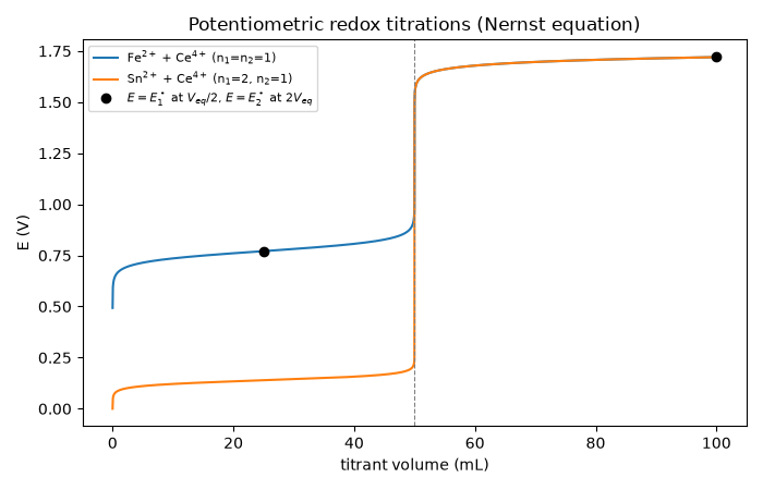
RedoxTitration computes the electrode potential during a redox titration from the Nernst equation, \(E=E^\circ-\frac{RT}{nF}\ln Q\): before equivalence the analyte couple sets E, after it the titrant couple does. At half-equivalence \(E=E^\circ_1\) exactly, at twice the equivalence volume \(E=E^\circ_2\), and the endpoint is read, as in the laboratory, at the steepest rise of E.

import matplotlib.pyplot as plt
import numpy as np

from chemistrykit.analytical import RedoxTitration

Fe2+ titrated by Ce4+ (both one-electron couples) – symmetric curve:

fe_ce = RedoxTitration(E1_standard=0.771, n1=1, E2_standard=1.72, n2=1, C_analyte=0.100, V_analyte=0.050, C_titrant=0.100)
V = np.linspace(1e-6, 0.099, 4000)
curve = fe_ce.curve(V)
V_eq = fe_ce.equivalence_volume()
E_half, E_eq, E_double = fe_ce.response_at(np.array([V_eq / 2, V_eq, 2 * V_eq]))
print(f"Equivalence volume: exact {V_eq * 1000:.3f} mL, steepest-rise estimate {fe_ce.find_equivalence_point(V) * 1000:.3f} mL")
print(f"E at V_eq/2  = {E_half:.4f} V  (E1 = 0.771 V)")
print(f"E at V_eq    = {E_eq:.4f} V  ((E1 + E2)/2 = {(0.771 + 1.72) / 2:.4f} V)")
print(f"E at 2 V_eq  = {E_double:.4f} V  (E2 = 1.72 V)")

Equivalence volume: exact 50.000 mL, steepest-rise estimate 50.008 mL
E at V_eq/2  = 0.7710 V  (E1 = 0.771 V)
E at V_eq    = 1.2455 V  ((E1 + E2)/2 = 1.2455 V)
E at 2 V_eq  = 1.7200 V  (E2 = 1.72 V)

The Nernst slope RT/(nF)*ln(10) = 59.16 mV per decade at 25 C: in the buffer region, every tenfold change in [Fe3+]/[Fe2+] moves E by 59 mV.

V_10 = V_eq * 10 / 11  # [Fe3+]/[Fe2+] = 10
V_1 = V_eq / 2  # ratio = 1
dE = fe_ce.response_at(np.array([V_10]))[0] - fe_ce.response_at(np.array([V_1]))[0]
print(f"\nE change for a tenfold ratio change: {dE * 1000:.2f} mV")

E change for a tenfold ratio change: 59.16 mV

An unequal-electron pair (a 2-electron analyte, e.g. Sn2+ -> Sn4+, titrated by 1-electron Ce4+) is asymmetric: E_eq = (2 E1 + E2)/3.

sn_ce = RedoxTitration(E1_standard=0.139, n1=2, E2_standard=1.72, n2=1, C_analyte=0.050, V_analyte=0.050, C_titrant=0.100)
curve_sn = sn_ce.curve(V)
print(f"\nSn2+/Ce4+ E_eq = {sn_ce.response_at(np.array([sn_ce.equivalence_volume()]))[0]:.4f} V (weighted mean {(2 * 0.139 + 1.72) / 3:.4f} V)")

Sn2+/Ce4+ E_eq = 0.6660 V (weighted mean 0.6660 V)

fig, ax = plt.subplots(figsize=(7, 4.5))
ax.plot(curve.V * 1000, curve.response, label="Fe$^{2+}$ + Ce$^{4+}$ (n$_1$=n$_2$=1)")
ax.plot(curve_sn.V * 1000, curve_sn.response, label="Sn$^{2+}$ + Ce$^{4+}$ (n$_1$=2, n$_2$=1)")
ax.axvline(V_eq * 1000, color="gray", linestyle="--", linewidth=0.8)
ax.plot([V_eq / 2 * 1000, 2 * V_eq * 1000], [E_half, E_double], "ko", label=r"$E=E^\circ_1$ at $V_{eq}/2$, $E=E^\circ_2$ at $2V_{eq}$")
ax.set_xlabel("titrant volume (mL)")
ax.set_ylabel("E (V)")
ax.set_title("Potentiometric redox titrations (Nernst equation)")
ax.legend(fontsize=8)
plt.tight_layout()
plt.show()