EDTA complexometric titration of a metal ion

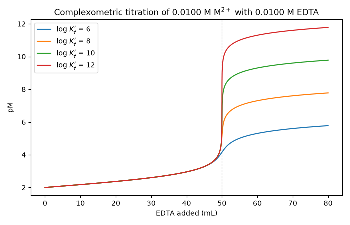
EDTATitration follows \(M+Y\rightleftharpoons MY\) through its conditional formation constant \(K_f'\). The same EDTA titrant quantifies any metal it binds strongly enough; the size of the pM break at equivalence is set by \(K_f'\), which is why Schwarzenbach’s titrations are run in a buffer at a pH where \(K_f'\) is large.

import matplotlib.pyplot as plt
import numpy as np

from chemistrykit.analytical import EDTATitration

V = np.linspace(1e-6, 0.080, 4000)
curves = {}
for logK in (6, 8, 10, 12):
    titration = EDTATitration(C_metal=0.0100, V_metal=0.050, K_conditional=10.0**logK, C_edta=0.0100)
    curves[logK] = titration.curve(V)
    V_eq = titration.equivalence_volume()
    pM_before, pM_eq, pM_after = titration.response_at(np.array([0.99 * V_eq, V_eq, 1.01 * V_eq]))
    C_M_eq = 0.0100 * 0.050 / (0.050 + V_eq)
    print(
        f"log K'={logK:2d}: pM at equivalence {pM_eq:.3f} (large-K approximation {0.5 * np.log10(10.0**logK / C_M_eq):.3f}), "
        f"jump over +/-1% of V_eq = {pM_after - pM_before:.2f} pM units, endpoint found at {titration.find_equivalence_point(V) * 1000:.2f} mL"
    )

log K'= 6: pM at equivalence 4.154 (large-K approximation 4.151), jump over +/-1% of V_eq = 0.30 pM units, endpoint found at 49.97 mL
log K'= 8: pM at equivalence 5.151 (large-K approximation 5.151), jump over +/-1% of V_eq = 1.72 pM units, endpoint found at 49.99 mL
log K'=10: pM at equivalence 6.151 (large-K approximation 6.151), jump over +/-1% of V_eq = 3.70 pM units, endpoint found at 49.99 mL
log K'=12: pM at equivalence 7.151 (large-K approximation 7.151), jump over +/-1% of V_eq = 5.70 pM units, endpoint found at 49.99 mL

fig, ax = plt.subplots(figsize=(7, 4.5))
for logK, curve in curves.items():
    ax.plot(curve.V * 1000, curve.response, label=f"log $K_f'$ = {logK}")
ax.axvline(50.0, color="gray", linestyle="--", linewidth=0.8)
ax.set_xlabel("EDTA added (mL)")
ax.set_ylabel("pM")
ax.set_title("Complexometric titration of 0.0100 M M$^{2+}$ with 0.0100 M EDTA")
ax.legend()
plt.tight_layout()
plt.show()