Pauling’s radius-ratio rule: predicting coordination numbers

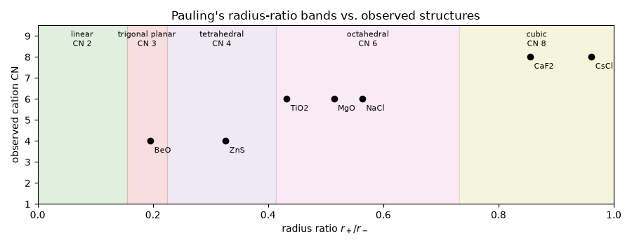
Pauling’s first rule (1929): each cation is surrounded by a polyhedron of anions whose size is fixed by the radius ratio \(r_+/r_-\). A polyhedron is stable only while the anions still touch the cation, which sets the limits \(\sqrt2-1=0.414\) (octahedral), \(\sqrt3-1=0.732\) (cubic), and so on. radius_ratio_coordination() applies the rule; here it is tested against observed structures.

import matplotlib.pyplot as plt

from chemistrykit.crystal.systems.crystal_chemistry import RADIUS_RATIO_LIMITS, radius_ratio_coordination

compounds = {
    # name: (r_cation, r_anion in pm, observed cation coordination)
    "BeO (wurtzite)": (27.0, 138.0, 4),  # Be2+ CN4, O2- CN4
    "ZnS (zinc blende)": (60.0, 184.0, 4),  # Zn2+ CN4, S2- CN6
    "NaCl (rock salt)": (102.0, 181.0, 6),
    "MgO (rock salt)": (72.0, 140.0, 6),
    "TiO2 (rutile)": (60.5, 140.0, 6),
    "CsCl": (174.0, 181.0, 8),  # Cs+ CN8
    "CaF2 (fluorite)": (112.0, 131.0, 8),  # Ca2+ CN8, F- CN4
}
print(f"{'compound':20s} {'r+/r-':>6s}  {'predicted':>20s}  observed CN")
hits = 0
for name, (rc, ra, observed) in compounds.items():
    p = radius_ratio_coordination(rc, ra)
    hits += p.coordination_number == observed
    print(f"{name:20s} {p.radius_ratio:6.3f}  {p.geometry:>14s} (CN {p.coordination_number})  {observed}")
print(f"\n{hits}/{len(compounds)} coordination numbers predicted correctly")

compound              r+/r-             predicted  observed CN
BeO (wurtzite)        0.196  trigonal planar (CN 3)  4
ZnS (zinc blende)     0.326     tetrahedral (CN 4)  4
NaCl (rock salt)      0.564      octahedral (CN 6)  6
MgO (rock salt)       0.514      octahedral (CN 6)  6
TiO2 (rutile)         0.432      octahedral (CN 6)  6
CsCl                  0.961           cubic (CN 8)  8
CaF2 (fluorite)       0.855           cubic (CN 8)  8

6/7 coordination numbers predicted correctly

The rule is a guide, not a law: BeO above falls just below the tetrahedral limit, and LiI (r+/r- = 0.35) is rock salt, not tetrahedral, because real ions are not hard spheres.

print(f"LiI: predicted CN {radius_ratio_coordination(76.0, 220.0).coordination_number}, observed CN 6")

LiI: predicted CN 4, observed CN 6

fig, ax = plt.subplots(figsize=(9, 3.5))
edges = [lim[0] for lim in RADIUS_RATIO_LIMITS] + [1.0]
for (lo, cn, geom), hi in zip(RADIUS_RATIO_LIMITS, edges[1:], strict=True):
    ax.axvspan(lo, hi, alpha=0.15, color=f"C{cn % 10}")
    ax.text((lo + hi) / 2.0, 9.3, f"{geom}\nCN {cn}", ha="center", va="top", fontsize=8)
for name, (rc, ra, observed) in compounds.items():
    ax.plot(rc / ra, observed, "ko")
    ax.annotate(name.split(" ")[0], (rc / ra, observed), textcoords="offset points", xytext=(4, -12), fontsize=8)
ax.set_xlim(0, 1.0)
ax.set_ylim(1, 9.5)
ax.set_xlabel(r"radius ratio $r_+/r_-$")
ax.set_ylabel("observed cation CN")
ax.set_title("Pauling's radius-ratio bands vs. observed structures")
plt.tight_layout()
plt.show()