Goldschmidt’s tolerance factor: which perovskites are cubic

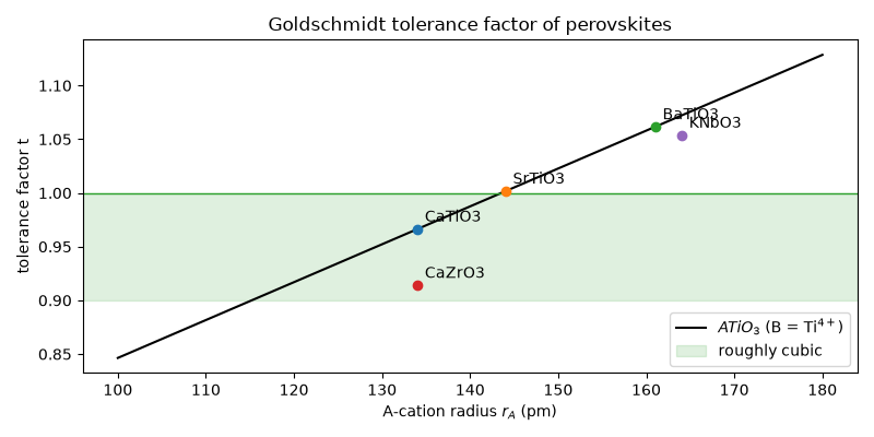
Goldschmidt (1926) noted that in an ideal cubic \(ABX_3\) perovskite the A-X distance equals \(\sqrt2\) times the B-X distance, so hard spheres fit exactly when \(t=(r_A+r_X)/[\sqrt2(r_B+r_X)]=1\) (goldschmidt_tolerance_factor()). Titanates with A-cations of different sizes span the range from tilted to cubic to ferroelectrically distorted.

import matplotlib.pyplot as plt
import numpy as np

from chemistrykit.crystal.systems.crystal_chemistry import goldschmidt_tolerance_factor

r_O = 140.0
perovskites = {
    # name: (r_A (CN 12), r_B (CN 6), observed room-temperature structure), Shannon radii in pm
    "CaTiO3": (134.0, 60.5, "orthorhombic (tilted)"),
    "SrTiO3": (144.0, 60.5, "cubic"),
    "BaTiO3": (161.0, 60.5, "tetragonal (ferroelectric)"),
    "CaZrO3": (134.0, 72.0, "orthorhombic (tilted)"),
    "KNbO3": (164.0, 64.0, "orthorhombic (ferroelectric)"),
}
ts = {}
for name, (r_a, r_b, observed) in perovskites.items():
    ts[name] = goldschmidt_tolerance_factor(r_a, r_b, r_O)
    print(f"{name:7s} t = {ts[name]:.3f}   observed: {observed}")
assert abs(ts["SrTiO3"] - 1.0) < 0.01
assert ts["CaTiO3"] < ts["SrTiO3"] < ts["BaTiO3"]

CaTiO3  t = 0.966   observed: orthorhombic (tilted)
SrTiO3  t = 1.002   observed: cubic
BaTiO3  t = 1.062   observed: tetragonal (ferroelectric)
CaZrO3  t = 0.914   observed: orthorhombic (tilted)
KNbO3   t = 1.054   observed: orthorhombic (ferroelectric)

r_a = np.linspace(100.0, 180.0, 200)
fig, ax = plt.subplots(figsize=(8, 4))
ax.plot(r_a, goldschmidt_tolerance_factor(r_a, 60.5, r_O), "k-", label=r"$ATiO_3$ (B = Ti$^{4+}$)")
ax.axhspan(0.9, 1.0, color="C2", alpha=0.15, label="roughly cubic")
ax.axhline(1.0, color="C2", lw=1)
for name, (r_a_i, _r_b, _) in perovskites.items():
    ax.plot(r_a_i, ts[name], "o")
    ax.annotate(name, (r_a_i, ts[name]), textcoords="offset points", xytext=(5, 5))
ax.set_xlabel(r"A-cation radius $r_A$ (pm)")
ax.set_ylabel("tolerance factor t")
ax.set_title("Goldschmidt tolerance factor of perovskites")
ax.legend(loc="lower right")
plt.tight_layout()
plt.show()