Tafel’s law: overpotential linear in log current

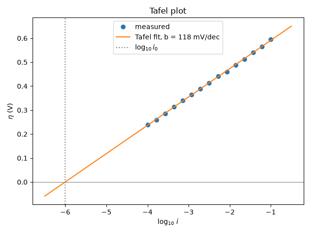
Tafel (1905) found that far from equilibrium the overpotential of hydrogen evolution grows linearly with \(\log_{10} i\): \(\eta = b\log_{10}(i/i_0)\). This example generates noisy “measured” high-overpotential data, draws the Tafel plot, and uses fit_tafel_plot() to recover the Tafel slope b and exchange current density \(i_0\) by linear regression – the analysis Tafel’s successors still use, and compares the slope with tafel_slope()’s textbook ~118 mV/decade for \(\alpha = 0.5\), n = 1.

import matplotlib.pyplot as plt
import numpy as np

from chemistrykit.electrochem.systems.butler_volmer import fit_tafel_plot, tafel_overpotential, tafel_slope

i0_true, alpha, n = 1.0e-6, 0.5, 1
b_true = tafel_slope(alpha=alpha, n=n)

Synthetic measurements: current densities over three decades, with the overpotential read to +/- 3 mV.

rng = np.random.default_rng(1905)
i_data = np.logspace(-4, -1, 15)
eta_data = tafel_overpotential(i_data, i0_true, alpha=alpha, n=n) + rng.normal(0.0, 0.003, i_data.size)
fit = fit_tafel_plot(eta_data, i_data)
print(f"true b  = {b_true * 1e3:.1f} mV/decade, fitted b  = {fit.tafel_slope * 1e3:.1f} mV/decade")
print(f"true i0 = {i0_true:.2e}, fitted i0 = {fit.exchange_current_density:.2e}, R^2 = {fit.r_squared:.4f}")

true b  = 118.3 mV/decade, fitted b  = 118.2 mV/decade
true i0 = 1.00e-06, fitted i0 = 9.95e-07, R^2 = 0.9995

The Tafel plot: a straight line whose extrapolation to eta = 0 gives log10(i0).

log_i = np.linspace(-6.5, -0.5, 100)
fig, ax = plt.subplots()
ax.plot(np.log10(i_data), eta_data, "o", label="measured")
ax.plot(log_i, fit.predict(10.0**log_i), label=f"Tafel fit, b = {fit.tafel_slope * 1e3:.0f} mV/dec")
ax.axhline(0.0, color="gray", linewidth=0.8)
ax.axvline(np.log10(fit.exchange_current_density), color="gray", linestyle=":", label=r"$\log_{10} i_0$")
ax.set_xlabel(r"$\log_{10}\, i$")
ax.set_ylabel(r"$\eta$ (V)")
ax.set_title("Tafel plot")
ax.legend()
fig.tight_layout()
plt.show()