The Butler-Volmer equation: anodic and cathodic partial currents

The Butler-Volmer equation writes the net electrode current as the difference of an anodic and a cathodic exponential. At zero overpotential the two partial currents are equal (each is \(i_0\)) and cancel – a dynamic equilibrium; far from equilibrium one term dominates and the equation becomes Tafel’s straight line. This example plots both partial currents and butler_volmer_current_density(), shows the effect of the transfer coefficient \(\alpha\), and checks numerically how fast the Tafel limit is reached.

import matplotlib.pyplot as plt
import numpy as np

from chemistrykit.constants import FARADAY, STANDARD_TEMPERATURE, R
from chemistrykit.electrochem.systems.butler_volmer import butler_volmer_current_density, tafel_overpotential
from chemistrykit.electrochem.visualizers.electrochem_plots import plot_tafel

i0, n = 1.0e-6, 1
f = n * FARADAY / (R * STANDARD_TEMPERATURE)
eta = np.linspace(-0.2, 0.2, 400)

Partial currents for alpha = 0.5 and the net current.

alpha = 0.5
i_a = i0 * np.exp(alpha * f * eta)
i_c = -i0 * np.exp(-(1 - alpha) * f * eta)
i_net = butler_volmer_current_density(i0, eta, alpha=alpha, n=n)
print(f"net current at eta = 0: {butler_volmer_current_density(i0, 0.0, alpha=alpha, n=n):.1e} (partial currents +/- {i0:.0e})")

fig, (ax1, ax2) = plt.subplots(1, 2, figsize=(10, 4))
ax1.plot(eta, i_a * 1e6, "--", label="anodic")
ax1.plot(eta, i_c * 1e6, "--", label="cathodic")
ax1.plot(eta, i_net * 1e6, "k", label="net (Butler-Volmer)")
ax1.set_ylim(-50, 50)
ax1.set_xlabel(r"$\eta$ (V)")
ax1.set_ylabel(r"$i$ ($\mu$A cm$^{-2}$)")
ax1.set_title(r"$\alpha$ = 0.5")
ax1.legend()

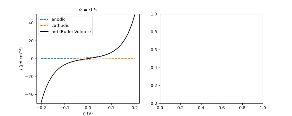
net current at eta = 0: 0.0e+00 (partial currents +/- 1e-06)

<matplotlib.legend.Legend object at 0x1195acad0>

The transfer coefficient skews the curve toward one branch.

for a in (0.3, 0.5, 0.7):
    ax2.plot(eta, butler_volmer_current_density(i0, eta, alpha=a, n=n) * 1e6, label=rf"$\alpha$ = {a}")
ax2.set_ylim(-50, 50)
ax2.set_xlabel(r"$\eta$ (V)")
ax2.set_title("Effect of the transfer coefficient")
ax2.legend()
fig.tight_layout()

High-overpotential limit: the Tafel form recovers eta from the full Butler-Volmer current with rapidly shrinking error.

for e in (0.05, 0.10, 0.20, 0.30):
    i_full = butler_volmer_current_density(i0, e, alpha=alpha, n=n)
    err = abs(tafel_overpotential(i_full, i0, alpha=alpha, n=n) - e) / e
    print(f"eta = {e:.2f} V: Tafel-limit relative error = {err:.2%}")

ax = plot_tafel(i0=i0, eta_range=(-0.4, 0.4), alpha=alpha, n=n)
plt.tight_layout()
plt.show()

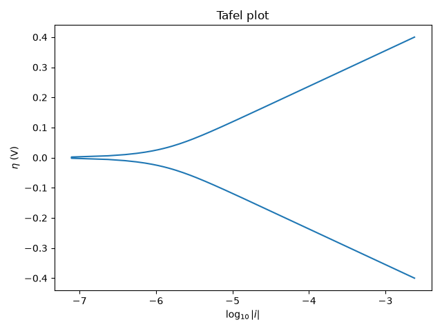
eta = 0.05 V: Tafel-limit relative error = 15.82%
eta = 0.10 V: Tafel-limit relative error = 1.04%
eta = 0.20 V: Tafel-limit relative error = 0.01%
eta = 0.30 V: Tafel-limit relative error = 0.02%