The Nernst equation: cell potential versus concentration

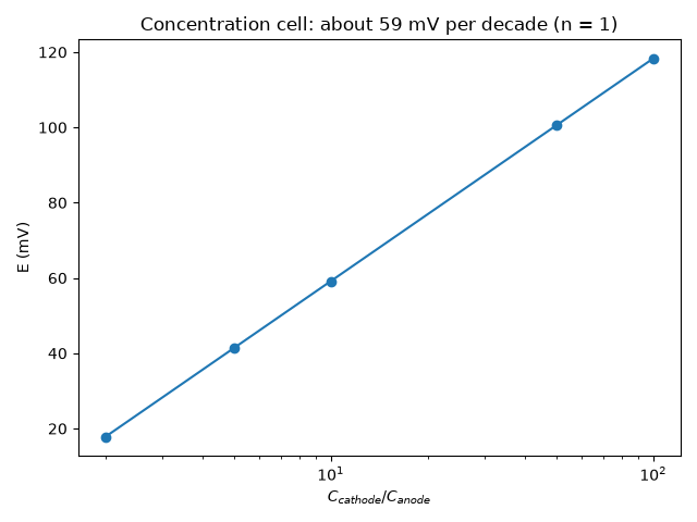
nernst_potential() implements \(E = E^\circ - \frac{RT}{nF}\ln Q\). This example checks that it reduces to \(E^\circ\) at \(Q=1\), plots the logarithmic dependence on the reaction quotient, and then builds a concentration cell (concentration_cell_potential()) whose voltage comes entirely from a concentration difference – about 59 mV per decade for a one-electron couple at 25 degC, as Nernst predicted.

import matplotlib.pyplot as plt
import numpy as np

from chemistrykit.electrochem.systems.nernst import concentration_cell_potential, nernst_potential
from chemistrykit.electrochem.visualizers.electrochem_plots import plot_nernst_concentration_dependence

E_standard, n = 0.34, 2  # Cu2+/Cu half-reaction vs. SHE
for Q in np.logspace(-3, 3, 7):
    print(f"Q={Q:9.3g}  E = {nernst_potential(E_standard, n, Q):+.4f} V")
print(f"\nNernst at Q=1: {nernst_potential(E_standard, n, Q=1.0)} V (= E_standard)")

ax = plot_nernst_concentration_dependence(E_standard=E_standard, n=n)
plt.tight_layout()

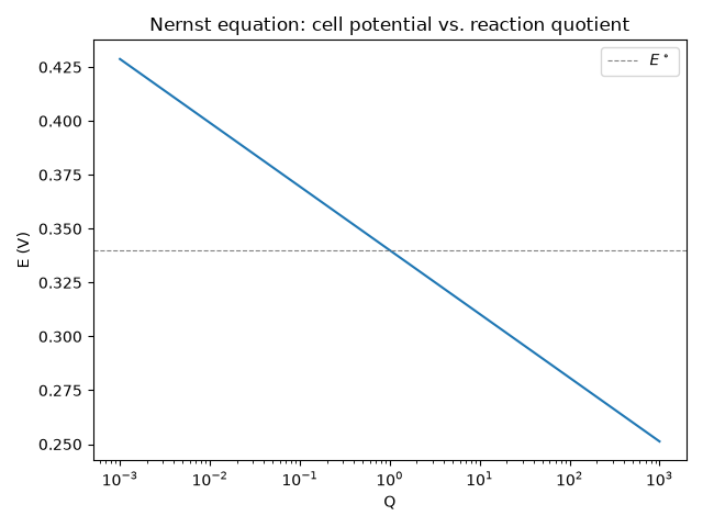
Q=    0.001  E = +0.4287 V
Q=     0.01  E = +0.3992 V
Q=      0.1  E = +0.3696 V
Q=        1  E = +0.3400 V
Q=       10  E = +0.3104 V
Q=      100  E = +0.2808 V
Q=    1e+03  E = +0.2513 V

Nernst at Q=1: 0.34 V (= E_standard)

A concentration cell: identical half-cells, E_standard = 0, so the voltage is pure Nernst term.

ratios = np.array([2.0, 5.0, 10.0, 50.0, 100.0])
E_conc = concentration_cell_potential(n=1, C_cathode=ratios * 0.01, C_anode=0.01)
fig, ax2 = plt.subplots()
ax2.plot(ratios, E_conc * 1e3, "o-")
ax2.set_xscale("log")
ax2.set_xlabel(r"$C_{cathode}/C_{anode}$")
ax2.set_ylabel("E (mV)")
ax2.set_title("Concentration cell: about 59 mV per decade (n = 1)")
fig.tight_layout()
plt.show()