Debye-Hückel activity corrections to the Nernst equation

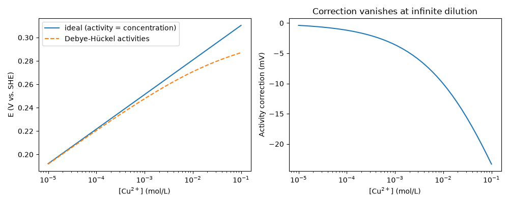
Debye and Hückel (1923) showed that each ion’s cloud of counter-ions lowers its activity below its concentration, by an amount growing with ionic strength and ionic charge. This example uses nernst_potential_with_activity() (built on chemistrykit.solutions.systems.activity) to show how the potential of a Cu2+/Cu electrode drifts away from the ideal Nernst value as the solution gets more concentrated, and that the correction vanishes in the dilute limit.

import matplotlib.pyplot as plt
import numpy as np

from chemistrykit.electrochem.systems.nernst import nernst_potential, nernst_potential_with_activity

Cu2+ + 2e- -> Cu(s) in CuSO4 solution: Q = 1/a(Cu2+). The sulfate counter-ion contributes to the ionic strength but not to Q (stoichiometric coefficient 0); the solid copper is at unit activity.

E_standard, n = 0.34, 2
c_cu = np.logspace(-5, -1, 40)
E_ideal = np.array([nernst_potential(E_standard, n, 1.0 / c) for c in c_cu])
E_dh = np.array([nernst_potential_with_activity(E_standard, n, [c, c, 1.0], [2, -2, 0], [-1.0, 0.0, 0.0]) for c in c_cu])

for c, e_i, e_a in zip(c_cu[::13], E_ideal[::13], E_dh[::13], strict=True):
    print(f"[Cu2+] = {c:8.1e} M: ideal E = {e_i:.4f} V, Debye-Hückel E = {e_a:.4f} V, shift = {1e3 * (e_a - e_i):+.2f} mV")

[Cu2+] =  1.0e-05 M: ideal E = 0.1921 V, Debye-Hückel E = 0.1917 V, shift = -0.38 mV
[Cu2+] =  2.2e-04 M: ideal E = 0.2315 V, Debye-Hückel E = 0.2298 V, shift = -1.72 mV
[Cu2+] =  4.6e-03 M: ideal E = 0.2710 V, Debye-Hückel E = 0.2638 V, shift = -7.22 mV
[Cu2+] =  1.0e-01 M: ideal E = 0.3104 V, Debye-Hückel E = 0.2871 V, shift = -23.33 mV

fig, (ax1, ax2) = plt.subplots(1, 2, figsize=(10, 4))
ax1.semilogx(c_cu, E_ideal, label="ideal (activity = concentration)")
ax1.semilogx(c_cu, E_dh, "--", label="Debye-Hückel activities")
ax1.set_xlabel(r"[Cu$^{2+}$] (mol/L)")
ax1.set_ylabel("E (V vs. SHE)")
ax1.legend()
ax2.semilogx(c_cu, 1e3 * (E_dh - E_ideal))
ax2.set_xlabel(r"[Cu$^{2+}$] (mol/L)")
ax2.set_ylabel("Activity correction (mV)")
ax2.set_title("Correction vanishes at infinite dilution")
fig.tight_layout()
plt.show()