Chain-branching explosions and Semenov’s critical condition

StoichiometricNetwork’s general mass-action engine, applied to a three-step radical chain mechanism (initiation, branching propagation, and linear termination), reproduces the qualitative signature of a chain-branching explosion: below a critical branching rate the radical concentration stays small and the fuel decays gently, while above it the radical population grows explosively and burns through the fuel in a short, sharp spike – exactly the ignition-vs-no-ignition switch behind Semenov’s and Hinshelwood’s explosion-limit theory.

import matplotlib.pyplot as plt

from chemistrykit.kinetics.systems.networks import StoichiometricNetwork
from chemistrykit.kinetics.visualizers.kinetics_plots import plot_concentration_vs_time

The mechanism: A -> 2R (initiation), A + R -> 2R + P (branching propagation, each radical that reacts produces two), and R -> P (linear, e.g. wall, termination). Species order (A, R, P); reaction order (initiation, branching, termination).

species = ("A", "R", "P")
stoich_matrix = [
    [-1.0, -1.0, 0.0],  # A
    [2.0, 1.0, -1.0],  # R
    [0.0, 1.0, 1.0],  # P
]
reactant_orders = [
    [1.0, 1.0, 0.0],  # A appears to first order in initiation and branching
    [0.0, 1.0, 1.0],  # R appears to first order in branching and termination
    [0.0, 0.0, 0.0],  # P is never a reactant
]

A0 = 1.0
k_i = 0.01
k_t = 2.0

Near the fuel concentration A0, the net radical growth rate is approximately d[R]/dt ~ (k_b*A0 - k_t)*[R] + 2*k_i*A0: a linear instability whose sign flips exactly at Semenov’s critical condition k_b*A0 = k_t. Two branching rate constants straddling that threshold give qualitatively different fates for the same fuel load.

cases = {
    "subcritical (k_b*A0 < k_t)": 0.5,
    "supercritical (k_b*A0 > k_t)": 5.0,
}

fig, axes = plt.subplots(1, 2, figsize=(11, 4.5))
for ax, (label, k_b) in zip(axes, cases.items()):
    rate_constants = [k_i, k_b, k_t]
    net = StoichiometricNetwork(species, stoich_matrix, rate_constants, reactant_orders, state0=[A0, 0.0, 0.0])
    result = net.integrate((0.0, 5.0), dt=1e-4, method="rk4")
    plot_concentration_vs_time(result, ax=ax)
    ax.set_title(f"{label}\nk_b={k_b}, k_b*A0={k_b * A0:g} vs k_t={k_t:g}")
    ax.set_ylim(-0.05, 1.05)

fig.suptitle("Chain-branching kinetics: the same fuel, two fates")
fig.tight_layout()

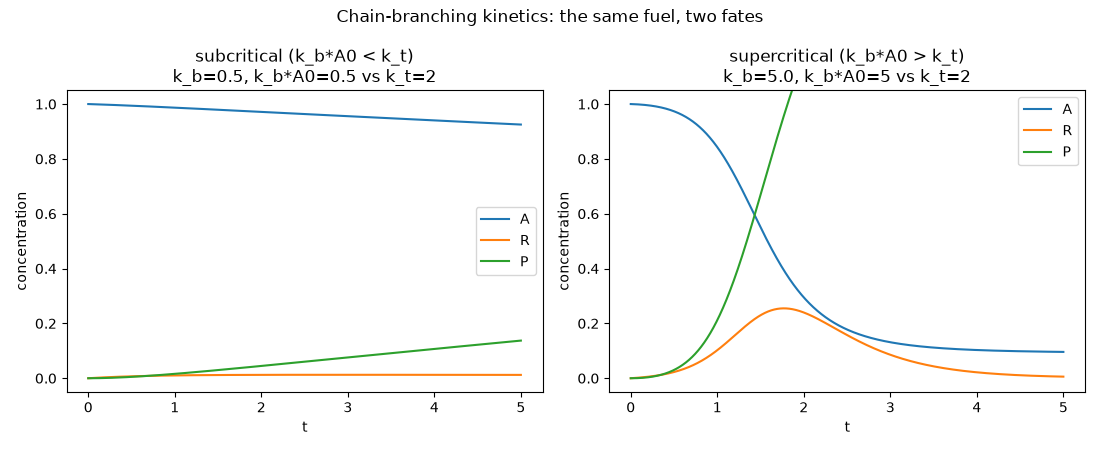
In the subcritical case the radical concentration relaxes to a small, quasi-steady value and the fuel decays slowly. In the supercritical case the radical population grows explosively – consuming essentially all of the fuel in a short, sharp burst – reproducing the qualitative ignition behavior behind the branching-chain explosion limits studied by Semenov and by Hinshelwood.

for label, k_b in cases.items():
    rate_constants = [k_i, k_b, k_t]
    net = StoichiometricNetwork(species, stoich_matrix, rate_constants, reactant_orders, state0=[A0, 0.0, 0.0])
    result = net.integrate((0.0, 5.0), dt=1e-4, method="rk4")
    peak_R = result.concentration("R").max()
    final_A = result.concentration("A")[-1]
    print(f"{label}: peak [R] = {peak_R:.4f}, final [A] = {final_A:.4f}")

plt.show()

subcritical (k_b*A0 < k_t): peak [R] = 0.0126, final [A] = 0.9253
supercritical (k_b*A0 > k_t): peak [R] = 0.2549, final [A] = 0.0960