Bateman’s closed-form solution for consecutive reactions

Bateman (1910) solved the chain of first-order steps \(A \xrightarrow{k_1} B \xrightarrow{k_2} C\) (written for radioactive decay series, but identical for consecutive chemical reactions) in closed form:

\[[B](t) = \frac{k_1 [A]_0}{k_2 - k_1}\left(e^{-k_1 t} - e^{-k_2 t}\right),\]

with the intermediate peaking at \(t_{max} = \ln(k_2/k_1)/(k_2 - k_1)\). consecutive_analytic() evaluates these formulas; here they are checked against a numerical integration of the same mechanism with StoichiometricNetwork.

import matplotlib.pyplot as plt
import numpy as np

from chemistrykit.kinetics.systems.networks import StoichiometricNetwork, consecutive_analytic
from chemistrykit.kinetics.visualizers.kinetics_plots import plot_concentration_vs_time

k1, k2, A0 = 1.0, 0.3, 1.0
net = StoichiometricNetwork.consecutive(k1=k1, k2=k2, A0=A0)
result = net.integrate((0.0, 15.0), dt=1e-3, method="rk4")
A_exact, B_exact, C_exact = consecutive_analytic(A0, k1, k2, result.t)
print(f"max |numeric - Bateman| for [B]: {np.max(np.abs(result.concentration('B') - B_exact)):.2e}")

fig, axes = plt.subplots(1, 2, figsize=(12, 4.5))
plot_concentration_vs_time(result, ax=axes[0])
for y in (A_exact, B_exact, C_exact):
    axes[0].plot(result.t, y, "k--", linewidth=0.8)
t_max = np.log(k2 / k1) / (k2 - k1)
axes[0].axvline(t_max, color="gray", linestyle=":", label=f"t_max = {t_max:.2f}")
axes[0].legend()
axes[0].set_title("A -> B -> C: numerical (solid) vs Bateman (dashed)")

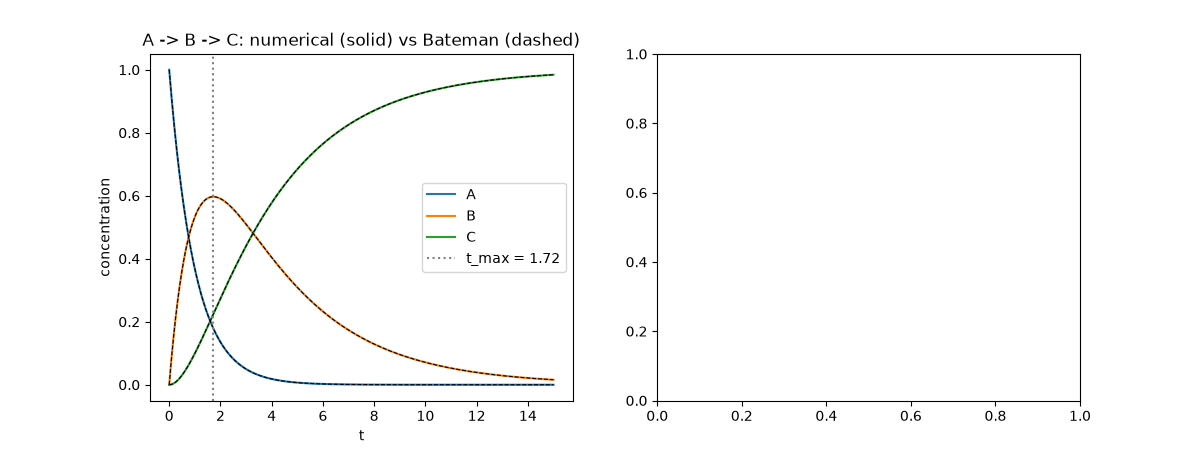
max |numeric - Bateman| for [B]: 4.44e-15

Text(0.5, 1.0, 'A -> B -> C: numerical (solid) vs Bateman (dashed)')

The height and timing of the intermediate’s peak depend only on the ratio of the two rate constants.

t = np.linspace(0.0, 15.0, 600)
for ratio in (0.1, 0.3, 1.0, 3.0, 10.0):
    _, B, _ = consecutive_analytic(A0=1.0, k1=1.0, k2=ratio, t=t)
    axes[1].plot(t, B, label=f"k2/k1 = {ratio:g}")
    if ratio != 1.0:
        tm = np.log(ratio) / (ratio - 1.0)
        _, Bm, _ = consecutive_analytic(1.0, 1.0, ratio, tm)
        axes[1].plot(tm, Bm, "ko", markersize=4)
axes[1].set_xlabel("t")
axes[1].set_ylabel("[B]")
axes[1].set_title("Intermediate peak at t_max = ln(k2/k1)/(k2-k1)")
axes[1].legend()

fig.tight_layout()
plt.show()