Eigen’s chemical relaxation: temperature jump and relaxation time

Eigen (1954) measured reactions far too fast to mix by perturbing an equilibrium mixture (a sudden temperature, pressure, or field jump) and timing its exponential return to the new equilibrium. For \(A \rightleftharpoons B\) the relaxation time is \(\tau = 1/(k_f + k_r)\), so combining \(\tau\) with the equilibrium constant \(K = k_f/k_r\) yields both rate constants. For the association \(A + B \rightleftharpoons C\) linearizing about equilibrium gives \(1/\tau = k_f([A]_{eq} + [B]_{eq}) + k_r\), the formula Eigen used to show that \(H^+ + OH^-\) recombination is diffusion-controlled.

import matplotlib.pyplot as plt
import numpy as np

from chemistrykit.kinetics.systems.networks import StoichiometricNetwork, reversible_analytic

Temperature jump on A <-> B: the mixture sits at equilibrium for the old rate constants; the jump changes them to (kf, kr) and the mixture relaxes with tau = 1/(kf + kr).

kf_old, kr_old = 1.0, 1.0
kf, kr = 3.0, 1.0
A_start = kr_old / (kf_old + kr_old)  # old equilibrium, total = 1
net = StoichiometricNetwork.reversible(kf=kf, kr=kr, A0=A_start, B0=1.0 - A_start)
result = net.integrate((0.0, 2.0), dt=1e-3, method="rk4")
A_eq = kr / (kf + kr)
tau = 1.0 / (kf + kr)
A_exact, _ = reversible_analytic(A_start, kf, kr, result.t, B0=1.0 - A_start)

fig, axes = plt.subplots(1, 3, figsize=(16, 4.5))
axes[0].plot(result.t, result.concentration("A"), color="steelblue", label="[A] numeric")
axes[0].plot(result.t, A_exact, "k--", linewidth=0.8, label="[A] analytic")
axes[0].axhline(A_eq, color="gray", linestyle=":", label="new [A]_eq")
axes[0].axvline(tau, color="crimson", linestyle=":", label=f"tau = 1/(kf+kr) = {tau:.2f}")
axes[0].set_xlabel("t after jump")
axes[0].set_ylabel("[A]")
axes[0].set_title("T-jump relaxation of A <-> B")
axes[0].legend()

deviation = np.abs(result.concentration("A") - A_eq)
mask = deviation > 1e-8
slope = np.polyfit(result.t[mask], np.log(deviation[mask]), 1)[0]
axes[1].semilogy(result.t, deviation, color="steelblue")
axes[1].set_xlabel("t after jump")
axes[1].set_ylabel("|[A] - [A]_eq|")
axes[1].set_title(f"Measured tau = {-1 / slope:.4f} (theory {tau:.4f})")

# Recover both rate constants from tau and K, as Eigen did.
K = (1.0 - A_eq) / A_eq
kr_rec = 1.0 / (-1 / slope * (K + 1.0))
print(f"recovered kf = {K * kr_rec:.4f} (true {kf}), kr = {kr_rec:.4f} (true {kr})")

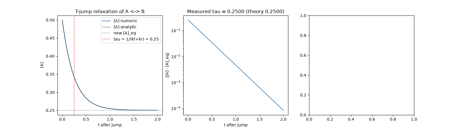
recovered kf = 3.0000 (true 3.0), kr = 1.0000 (true 1.0)

Association A + B <-> C: small perturbations about equilibrium decay with 1/tau = kf([A]_eq + [B]_eq) + kr, which grows with concentration.

kf2, kr2 = 5.0, 1.0
species = ("A", "B", "C")
stoich = [[-1.0, 1.0], [-1.0, 1.0], [1.0, -1.0]]
orders = [[1.0, 0.0], [1.0, 0.0], [0.0, 1.0]]
totals = np.array([0.05, 0.1, 0.2, 0.5, 1.0, 2.0])
inv_tau_meas, inv_tau_theory = [], []
for c_tot in totals:
    # equilibrium with [A]=[B]=x, [C]=c_tot-x: kf x^2 = kr (c_tot - x)
    x = (-kr2 + np.sqrt(kr2**2 + 4 * kf2 * kr2 * c_tot)) / (2 * kf2)
    delta = 1e-3 * x
    net2 = StoichiometricNetwork(species, stoich, [kf2, kr2], orders, state0=[x + delta, x + delta, c_tot - x - delta])
    res2 = net2.integrate((0.0, 3.0 / (2 * kf2 * x + kr2)), dt=1e-4, method="rk4")
    dev = res2.concentration("C") - (c_tot - x)
    good = np.abs(dev) > 1e-3 * np.abs(dev[0])
    inv_tau_meas.append(-np.polyfit(res2.t[good], np.log(np.abs(dev[good])), 1)[0])
    inv_tau_theory.append(kf2 * 2 * x + kr2)

axes[2].plot(totals, inv_tau_theory, color="darkorange", label=r"$k_f([A]_{eq}+[B]_{eq}) + k_r$")
axes[2].plot(totals, inv_tau_meas, "o", color="steelblue", label="measured from integration")
axes[2].set_xlabel("total concentration")
axes[2].set_ylabel(r"$1/\tau$")
axes[2].set_title("A + B <-> C: relaxation speeds up with concentration")
axes[2].legend()

fig.tight_layout()
plt.show()