Lotka’s autocatalytic oscillator and its neutral orbits

Lotka’s 1920 chemical scheme, with the reservoir \(A\) held constant,

\[A + X \xrightarrow{k_1} 2X, \qquad X + Y \xrightarrow{k_2} 2Y, \qquad Y \xrightarrow{k_3} P,\]

gives \(dX/dt = k_1[A]X - k_2XY\) and \(dY/dt = k_2XY - k_3Y\): concentrations oscillate forever with no external clock. But the orbits are only neutrally stable: the quantity

\[V = k_2 X - k_3 \ln X + k_2 Y - k_1[A] \ln Y\]

is conserved, so every starting point lies on its own closed curve and a perturbation simply moves the system to a different orbit. The mechanism is integrated here with the general mass-action engine StoichiometricNetwork.

import matplotlib.pyplot as plt
import numpy as np

from chemistrykit.kinetics.systems.networks import StoichiometricNetwork

k1A, k2, k3 = 1.0, 1.0, 1.0  # k1*[A] folded into a pseudo-first-order constant
species = ("X", "Y", "P")
stoich = [[1.0, -1.0, 0.0], [0.0, 1.0, -1.0], [0.0, 0.0, 1.0]]
orders = [[1.0, 1.0, 0.0], [0.0, 1.0, 1.0], [0.0, 0.0, 0.0]]


def lotka_invariant(X, Y):
    return k2 * X - k3 * np.log(X) + k2 * Y - k1A * np.log(Y)


fig, axes = plt.subplots(1, 3, figsize=(16, 4.5))
for X0, color in [(1.2, "steelblue"), (1.6, "darkorange"), (2.2, "seagreen"), (3.0, "crimson")]:
    net = StoichiometricNetwork(species, stoich, [k1A, k2, k3], orders, state0=[X0, 1.0, 0.0])
    result = net.integrate((0.0, 20.0), dt=1e-3, method="rk4")
    X, Y = result.concentration("X"), result.concentration("Y")
    axes[0].plot(X, Y, color=color, label=f"X0 = {X0}")
    V = lotka_invariant(X, Y)
    axes[1].plot(result.t, V - V[0], color=color)
    print(f"X0={X0}: relative drift of the invariant V = {np.ptp(V) / abs(V[0]):.1e}")
    if X0 == 2.2:
        axes[2].plot(result.t, X, color="steelblue", label="[X]")
        axes[2].plot(result.t, Y, color="darkorange", label="[Y]")

axes[0].plot(k3 / k2, k1A / k2, "k*", markersize=12, label="fixed point (neutral centre)")
axes[0].set_xlabel("[X]")
axes[0].set_ylabel("[Y]")
axes[0].set_title("A nested family of closed orbits")
axes[0].legend(fontsize=8)
axes[1].set_xlabel("t")
axes[1].set_ylabel("V(t) - V(0)")
axes[1].set_title("The conserved quantity V (no attracting cycle)")
axes[2].set_xlabel("t")
axes[2].set_ylabel("concentration")
axes[2].set_title("Undamped oscillation, X0 = 2.2")
axes[2].legend()
fig.tight_layout()

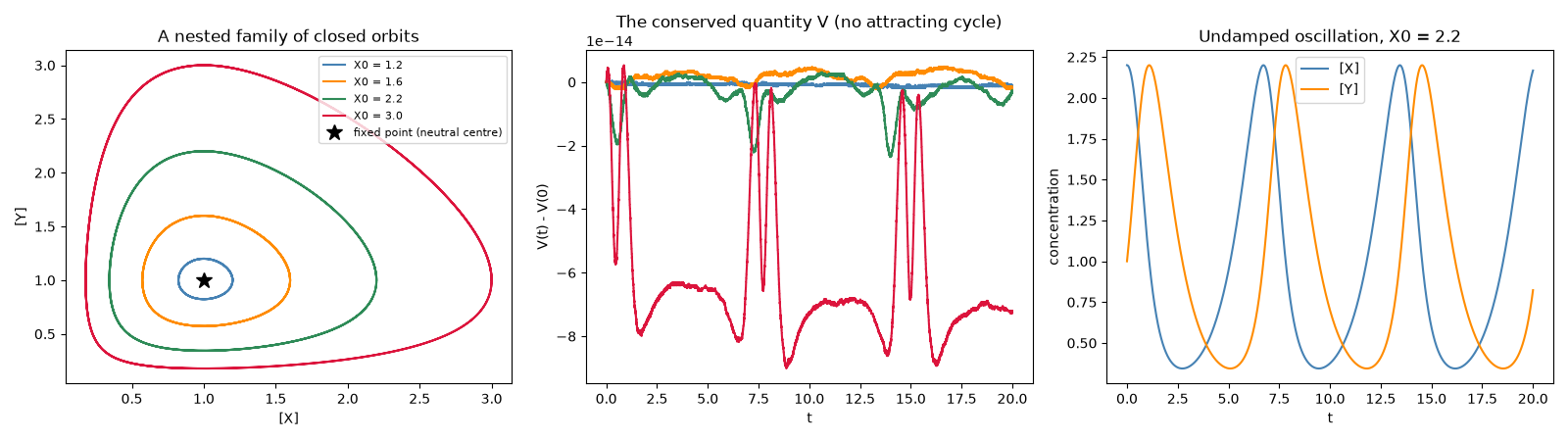
X0=1.2: relative drift of the invariant V = 1.1e-15
X0=1.6: relative drift of the invariant V = 3.3e-15
X0=2.2: relative drift of the invariant V = 1.1e-14
X0=3.0: relative drift of the invariant V = 3.3e-14

Contrast with the Brusselator (a genuine limit cycle): there, orbits started at different points converge to one amplitude; here each amplitude persists forever.

plt.show()