Eyring’s transition-state theory: activation enthalpy and entropy

Transition-state theory (Eyring; Evans and Polanyi, 1935) writes a rate constant as a universal frequency times an equilibrium constant for forming the activated complex,

\[k = \frac{k_BT}{h}\,e^{\Delta S^{\ddagger}/R}\,e^{-\Delta H^{\ddagger}/RT}.\]

Plotting \(\ln(k/T)\) against \(1/T\) (an “Eyring plot”) gives \(\Delta H^{\ddagger}\) from the slope and \(\Delta S^{\ddagger}\) from the intercept – giving the Arrhenius \(E_a\) and \(A\) a thermodynamic meaning. Here synthetic data generated with eyring_rate_constant() are fitted with fit_eyring() and, for comparison, fit_arrhenius().

import matplotlib.pyplot as plt
import numpy as np

from chemistrykit.constants import K_B, H, R
from chemistrykit.kinetics.systems.arrhenius import fit_arrhenius
from chemistrykit.kinetics.systems.rate_theory import eyring_rate_constant, fit_eyring

dH_true, dS_true = 85e3, -25.0  # J/mol, J/(mol K)
T = np.linspace(290.0, 350.0, 10)
rng = np.random.default_rng(1935)
k = eyring_rate_constant(T, dH_true, dS_true) * (1.0 + rng.normal(0.0, 0.02, T.shape))

eyring = fit_eyring(T, k)
arrhenius = fit_arrhenius(T, k)
T_mid = 1.0 / np.mean(1.0 / T)
print(f"true:    dH = {dH_true / 1000:.1f} kJ/mol, dS = {dS_true:.1f} J/(mol K)")
print(f"fitted:  dH = {eyring.dH / 1000:.1f} kJ/mol, dS = {eyring.dS:.1f} J/(mol K), dG(298) = {eyring.dG(298.15) / 1000:.1f} kJ/mol")
print(f"Arrhenius Ea = {arrhenius.Ea / 1000:.1f} kJ/mol  vs  dH + R*T = {(eyring.dH + R * T_mid) / 1000:.1f} kJ/mol")
print(f"Arrhenius A  = {arrhenius.A:.2e} /s vs e*kB*T/h*exp(dS/R) = {np.e * K_B * T_mid / H * np.exp(eyring.dS / R):.2e} /s")

fig, axes = plt.subplots(1, 2, figsize=(12, 4.5))
axes[0].plot(1.0 / T, np.log(k / T), "o", color="steelblue", label="data")
axes[0].plot(1.0 / T, np.log(eyring.predict(T) / T), color="darkorange", label=r"fit: slope $-\Delta H^{\ddagger}/R$")
axes[0].set_xlabel("1/T (1/K)")
axes[0].set_ylabel("ln(k/T)")
axes[0].set_title(f"Eyring plot: dH = {eyring.dH / 1000:.1f} kJ/mol, dS = {eyring.dS:.0f} J/(mol K)")
axes[0].legend()

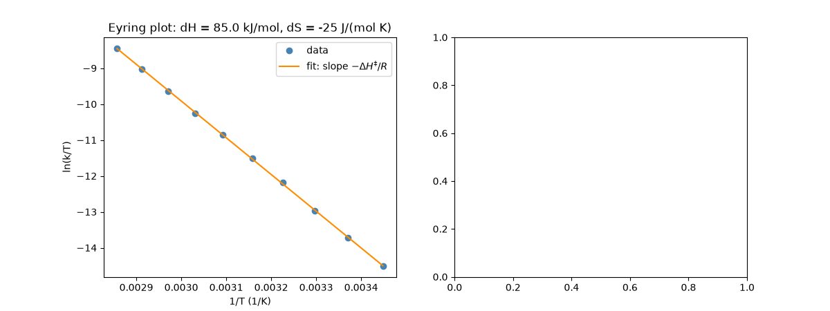
true:    dH = 85.0 kJ/mol, dS = -25.0 J/(mol K)
fitted:  dH = 85.0 kJ/mol, dS = -25.0 J/(mol K), dG(298) = 92.5 kJ/mol
Arrhenius Ea = 87.7 kJ/mol  vs  dH + R*T = 87.7 kJ/mol
Arrhenius A  = 8.96e+11 /s vs e*kB*T/h*exp(dS/R) = 8.96e+11 /s

<matplotlib.legend.Legend object at 0x11c732510>

The universal frequency k_B T/h (~6e12 /s) is the rate a reaction with no free-energy barrier would have; the barrier Delta G divides it down.

dG = np.linspace(0.0, 120e3, 200)
axes[1].semilogy(dG / 1000, K_B * 298.15 / H * np.exp(-dG / (R * 298.15)), color="steelblue")
axes[1].axvline(eyring.dG(298.15) / 1000, color="crimson", linestyle=":", label="fitted barrier at 298 K")
axes[1].set_xlabel(r"$\Delta G^{\ddagger}$ (kJ/mol)")
axes[1].set_ylabel("k at 298 K (1/s)")
axes[1].set_title("Rate constant set by the free-energy barrier")
axes[1].legend()

fig.tight_layout()
plt.show()