Lindemann-Hinshelwood falloff of a unimolecular rate constant

A unimolecular decomposition needs collisions to energize the molecule, so its first-order rate constant depends on pressure. LindemannHinshelwood gives the steady-state result \(k_{uni}=k_1k_2[M]/(k_{-1}[M]+k_2)\). It rises linearly at low pressure, where activation is the bottleneck, saturates at \(k_\infty=k_1k_2/k_{-1}\) at high pressure, and falls to half of \(k_\infty\) at \([M]_{1/2}=k_2/k_{-1}\). Left: the falloff curve, checked against a direct integration of the full three-step mechanism (network()). Right: Lindemann’s linearization \(1/k_{uni}\) against \(1/[M]\). Real data curve away from this straight line, the discrepancy that led to Hinshelwood’s, and later RRK and RRKM, energy-dependent \(k_2\).

import matplotlib.pyplot as plt
import numpy as np

from chemistrykit.kinetics import LindemannHinshelwood

lh = LindemannHinshelwood(k1=0.1, k_minus1=10.0, k2=100.0)
M = np.logspace(-1, 4, 200)

# Integrate the full mechanism for several [M]; the step must resolve A*'s
# lifetime 1/(k_-1[M] + k2), and the run lasts about 8 lifetimes of A.
M_check = np.array([0.3, 3.0, 30.0, 300.0])
k_numeric = []
for m in M_check:
    dt = 0.2 / (lh.k_minus1 * m + lh.k2)
    result = lh.network(m).integrate((0.0, 8.0 / float(lh.rate_constant(m))), dt=dt)
    A, t = result.concentration("A"), result.t
    i = len(t) // 2
    k_numeric.append(-np.log(A[-1] / A[i]) / (t[-1] - t[i]))

fig, axes = plt.subplots(1, 2, figsize=(12, 4.8))
axes[0].loglog(M, lh.rate_constant(M), color="darkorange", label=r"steady-state $k_{uni}$")
axes[0].loglog(M, lh.k0 * M, ":", color="gray", label=r"low-pressure limit $k_1[M]$")
axes[0].axhline(lh.k_inf, color="gray", linestyle="--", label=r"$k_\infty$")
axes[0].axvline(lh.M_half, color="steelblue", linewidth=0.8, label=r"$[M]_{1/2}$")
axes[0].loglog(M_check, k_numeric, "ko", label="full mechanism, integrated")
axes[0].set_xlabel("bath-gas concentration [M]")
axes[0].set_ylabel(r"$k_{uni}$ (s$^{-1}$)")
axes[0].set_title("Pressure falloff")
axes[0].legend()

inv_M = 1.0 / M
axes[1].plot(inv_M, lh.inverse_rate_constant(M), color="darkorange")
axes[1].set_xlim(0, 1.0)
axes[1].set_ylim(0, lh.inverse_rate_constant(1.0) * 1.05)
axes[1].set_xlabel("1/[M]")
axes[1].set_ylabel(r"$1/k_{uni}$ (s)")
axes[1].set_title(r"Lindemann plot: intercept $1/k_\infty$, slope $1/k_1$")
fig.tight_layout()

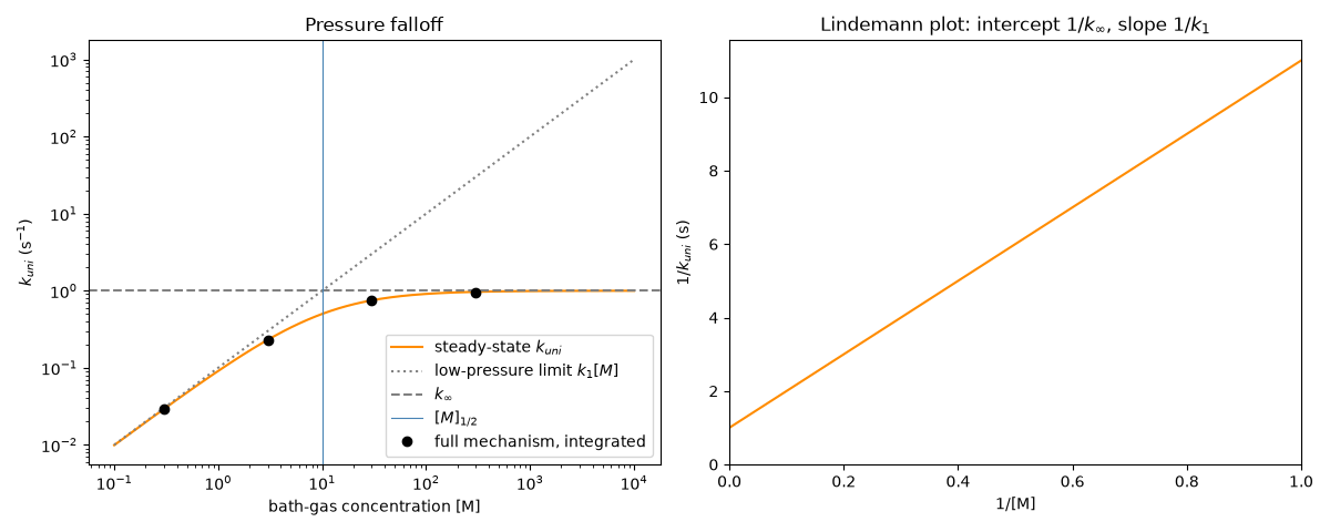
The two agree to within the steady-state approximation’s own error, of order \(k_1[M]/(k_{-1}[M]+k_2)\), about 1% here.

for m, k in zip(M_check, k_numeric, strict=True):
    print(f"[M] = {m:7.1f}: steady state {float(lh.rate_constant(m)):.4f}, integrated {k:.4f} s^-1")

plt.show()

[M] =     0.3: steady state 0.0291, integrated 0.0291 s^-1
[M] =     3.0: steady state 0.2308, integrated 0.2306 s^-1
[M] =    30.0: steady state 0.7500, integrated 0.7458 s^-1
[M] =   300.0: steady state 0.9677, integrated 0.9588 s^-1