Weeks-Chandler-Andersen: repulsive forces set the structure of a dense liquid

Weeks, Chandler, and Andersen split the Lennard-Jones potential at its minimum \(r_m=2^{1/6}\sigma\) into a purely repulsive reference part \(u_0\) and a smooth attractive perturbation \(w\):

\[\begin{split}u_0(r) = \begin{cases} u(r) + \epsilon, & r < r_m \\ 0, & r \ge r_m \end{cases} \qquad w(r) = \begin{cases} -\epsilon, & r < r_m \\ u(r), & r \ge r_m \end{cases}\end{split}\]

and showed that at liquid densities the structure of the full fluid is almost the same as that of the repulsive reference fluid alone. This example draws the split, then simulates both fluids with LJFluid at a dense liquid state point near the triple point (\(\rho^*=0.84\), \(T^*=0.75\)) – the full potential with the usual cutoff \(2.5\sigma\), the WCA reference by cutting at r_min – and compares their radial distribution functions.

import matplotlib.pyplot as plt
import numpy as np

from chemistrykit.md.systems.lj_fluid import LennardJones, LJFluid
from chemistrykit.md.systems.thermostats import VelocityRescalingThermostat

lj = LennardJones()
r_m = lj.r_min
r = np.linspace(0.9, 2.5, 400)
u = lj.energy(r)
u0 = np.where(r < r_m, u + 1.0, 0.0)
w = np.where(r < r_m, -1.0, u)

fig, axes = plt.subplots(1, 2, figsize=(11, 4.5))
axes[0].plot(r, u, color="black", label="full LJ  u = u0 + w")
axes[0].plot(r, u0, color="darkorange", linestyle="--", label="repulsive reference u0")
axes[0].plot(r, w, color="steelblue", linestyle="--", label="attractive perturbation w")
axes[0].axvline(r_m, color="gray", linestyle=":", linewidth=0.8)
axes[0].set_ylim(-1.3, 2.0)
axes[0].set_xlabel(r"r / $\sigma$")
axes[0].set_ylabel(r"energy / $\epsilon$")
axes[0].set_title("The WCA split at the potential minimum")
axes[0].legend()

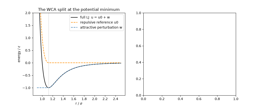
<matplotlib.legend.Legend object at 0x11ccfcd70>

Now the two fluids at the same dense state point. Each is equilibrated with a velocity-rescaling thermostat and g(r) is averaged over an NVE production run.

density, T = 0.84, 0.75
g_curves = {}
for label, cutoff, color in [("full LJ (cutoff 2.5 sigma)", 2.5, "black"), ("WCA repulsive reference", r_m, "darkorange")]:
    fluid = LJFluid.from_lattice(n_per_side=7, density=density, temperature=T, cutoff=cutoff, rng=0)
    fluid.run(dt=0.004, n_steps=3000, thermostat=VelocityRescalingThermostat(T, interval=10), sample_every=3000)
    result = fluid.run(dt=0.004, n_steps=1500, thermostat=VelocityRescalingThermostat(T, interval=10), sample_every=100)
    rr, _ = fluid.radial_distribution_function(n_bins=120)
    g = np.mean([fluid.radial_distribution_function(n_bins=120, positions=p)[1] for p in result.positions], axis=0)
    g_curves[label] = g
    axes[1].plot(rr, g, color=color, label=label)

axes[1].axhline(1.0, color="gray", linestyle=":", linewidth=0.8)
axes[1].set_xlabel(r"r / $\sigma$")
axes[1].set_ylabel("g(r)")
axes[1].set_title(rf"Dense liquid, $\rho^*$={density}, $T^*$={T}")
axes[1].legend()
fig.tight_layout()

The two radial distribution functions nearly coincide: removing the entire attractive tail barely changes where the neighbors sit, because in a dense liquid the attractions from all sides roughly cancel and the packing is dictated by the repulsive cores.

g_full, g_wca = g_curves.values()
print(f"first-peak height: full LJ {g_full.max():.2f}, WCA reference {g_wca.max():.2f}")
print(f"largest pointwise difference in g(r): {np.max(np.abs(g_full - g_wca)):.2f}")

plt.show()

first-peak height: full LJ 2.94, WCA reference 2.97
largest pointwise difference in g(r): 0.27