Flory’s steady-state kinetics of free-radical polymerization

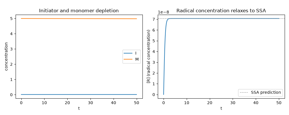
free_radical_network() builds the lumped initiation/propagation/termination kinetics as a StoichiometricNetwork and integrates it numerically. Because termination is much faster than initiator decomposition, the radical concentration relaxes almost immediately to the steady-state approximation’s closed-form prediction (steady_state_radical_concentration()) – verified here by comparing the two directly – while monomer is consumed only slowly, at the classic square-root-of-initiator rate.

import matplotlib.pyplot as plt
import numpy as np

from chemistrykit.polymer.systems.chain_growth import (
    free_radical_network,
    steady_state_radical_concentration,
    steady_state_rate_of_polymerization,
)
from chemistrykit.polymer.visualizers.polymer_plots import plot_free_radical_kinetics

kd, f, kp, kt = 1.0e-5, 0.5, 1.0e3, 1.0e7
I0, M0 = 0.01, 5.0

net = free_radical_network(kd, f, kp, kt, I0, M0)
result = net.integrate((0.0, 50.0), dt=1e-2, method="rk4")

R_ss = steady_state_radical_concentration(kd, f, I0, kt)
R_numeric_final = result.concentration("R")[-1]
print(f"SSA radical concentration:        {R_ss:.4e}")
print(f"Numerically integrated R(t=50):    {R_numeric_final:.4e}")
print(f"Relative difference: {abs(R_numeric_final - R_ss) / R_ss:.2%}")

SSA radical concentration:        7.0711e-08
Numerically integrated R(t=50):    7.0702e-08
Relative difference: 0.01%

The rate of polymerization scales as sqrt([I]), a distinctive signature of free-radical (vs. e.g. ionic) chain polymerization.

I_values = np.array([0.0025, 0.01, 0.04, 0.16])
Rp_values = steady_state_rate_of_polymerization(kd, f, kp, kt, I=I_values, M=M0)
print("\n[I]      Rp           Rp/sqrt([I])")
for I_val, Rp in zip(I_values, Rp_values):
    print(f"{I_val:<8} {Rp:<12.4e} {Rp / np.sqrt(I_val):.4e}")

[I]      Rp           Rp/sqrt([I])
0.0025   1.7678e-04   3.5355e-03
0.01     3.5355e-04   3.5355e-03
0.04     7.0711e-04   3.5355e-03
0.16     1.4142e-03   3.5355e-03

fig, axes = plt.subplots(1, 2, figsize=(10, 4))
plot_free_radical_kinetics(result, species=("I", "M"), ax=axes[0])
axes[0].set_title("Initiator and monomer depletion")

axes[1].plot(result.t, result.concentration("R"))
axes[1].axhline(R_ss, color="gray", linestyle="--", linewidth=0.8, label="SSA prediction")
axes[1].set_xlabel("t")
axes[1].set_ylabel("[R] (radical concentration)")
axes[1].set_title("Radical concentration relaxes to SSA")
axes[1].legend()
plt.tight_layout()
plt.show()