Combination vs. disproportionation termination

free_radical_network()’s mode argument selects between the two ways two growing radical chains can terminate: combination (they fuse into a single dead chain) or disproportionation (one radical abstracts a hydrogen from the other, producing two separate dead chains). Bevington, Melville, and Taylor (“The Termination Reaction in Radical Polymerizations,” J. Polym. Sci. 12 (1954), 449-459) showed how to distinguish the two experimentally, by end-group analysis and by the resulting degree of polymerization’s relationship to the kinetic chain length (kinetic_chain_length()) nu: \(\bar X_n = 2\nu\) for combination (two radicals’ worth of monomer per dead chain) but \(\bar X_n = \nu\) for disproportionation (one radical’s worth per dead chain) – verified here directly against the numerically integrated network.

import matplotlib.pyplot as plt
import numpy as np

from chemistrykit.polymer.systems.chain_growth import free_radical_network, kinetic_chain_length
from chemistrykit.polymer.visualizers.polymer_plots import plot_free_radical_kinetics

kd, f, kp, kt = 1.0e-5, 0.5, 1.0e3, 1.0e7
I0, M0 = 0.01, 5.0
t_span = (0.0, 50.0)

results = {
    mode: free_radical_network(kd, f, kp, kt, I0, M0, mode=mode).integrate(t_span, dt=1e-2, method="rk4") for mode in ("combination", "disproportionation")
}

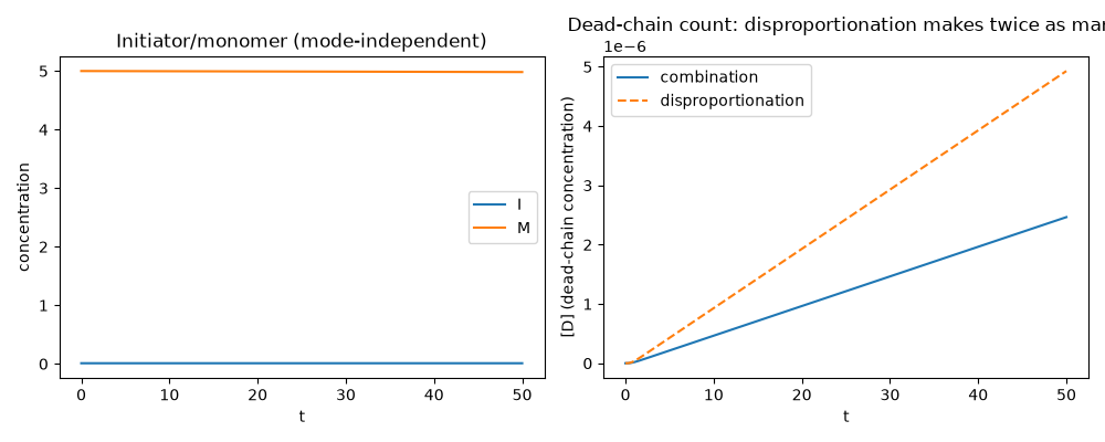
Radical, initiator, and monomer trajectories are identical between the two modes (only the dead-polymer bookkeeping differs); the dead-chain count D(t), however, is exactly twice as large for disproportionation as for combination at every instant, since each termination event (rate k_t[R]^2, the same in both modes) produces two dead chains instead of one.

D_comb = results["combination"].concentration("D")[-1]
D_dispro = results["disproportionation"].concentration("D")[-1]
print(f"D(t=50), combination:        {D_comb:.6e}")
print(f"D(t=50), disproportionation: {D_dispro:.6e}")
print(f"Ratio (should be exactly 2): {D_dispro / D_comb:.6f}")

D(t=50), combination:        2.464337e-06
D(t=50), disproportionation: 4.928673e-06
Ratio (should be exactly 2): 2.000000

The number-average degree of polymerization of the dead polymer – total monomer consumed divided by total dead chains formed – matches the kinetic-chain-length prediction: Xn = 2*nu for combination, Xn = nu for disproportionation.

nu = kinetic_chain_length(kd, f, kp, kt, I=I0, M=M0)
for mode in ("combination", "disproportionation"):
    result = results[mode]
    monomer_consumed = M0 - result.concentration("M")[-1]
    D_final = result.concentration("D")[-1]
    Xn_sim = monomer_consumed / D_final
    Xn_theory = 2.0 * nu if mode == "combination" else nu
    print(f"\n{mode}:")
    print(f"  Xn (simulated, monomer consumed / dead chains) = {Xn_sim:.1f}")
    print(f"  Xn (theory)                                    = {Xn_theory:.1f}")

combination:
  Xn (simulated, monomer consumed / dead chains) = 7090.2
  Xn (theory)                                    = 7071.1

disproportionation:
  Xn (simulated, monomer consumed / dead chains) = 3545.1
  Xn (theory)                                    = 3535.5

fig, axes = plt.subplots(1, 2, figsize=(10, 4))
plot_free_radical_kinetics(results["combination"], species=("I", "M"), ax=axes[0])
axes[0].set_title("Initiator/monomer (mode-independent)")

for mode, style in (("combination", "-"), ("disproportionation", "--")):
    axes[1].plot(results[mode].t, results[mode].concentration("D"), style, label=mode)
axes[1].set_xlabel("t")
axes[1].set_ylabel("[D] (dead-chain concentration)")
axes[1].set_title("Dead-chain count: disproportionation makes twice as many")
axes[1].legend()
plt.tight_layout()
plt.show()

assert np.isclose(D_dispro / D_comb, 2.0, rtol=1e-6)