The Mayo-Lewis copolymer equation: composition vs. feed

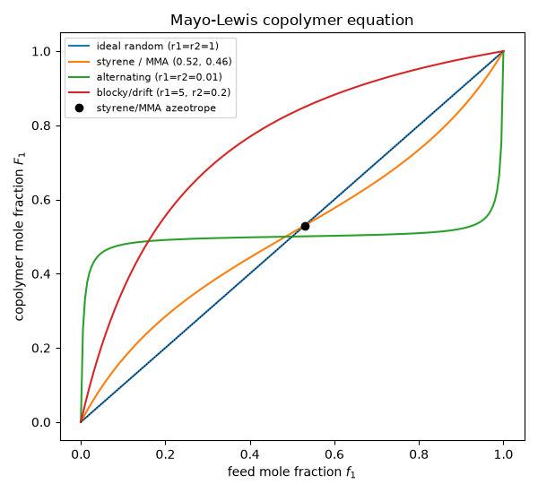
Mayo and Lewis (1944) showed that, if a growing radical’s reactivity depends only on its terminal monomer unit, the instantaneous copolymer composition \(F_1\) follows from the feed composition \(f_1\) and two reactivity ratios (mayo_lewis_copolymer_composition()). Their own test case, styrene / methyl methacrylate (\(r_1\approx0.52\), \(r_2\approx0.46\)), crosses the diagonal at an azeotropic feed (azeotropic_feed_composition()) where the copolymer has the same composition as the feed.

import matplotlib.pyplot as plt
import numpy as np

from chemistrykit.polymer.systems.copolymerization import (
    azeotropic_feed_composition,
    mayo_lewis_copolymer_composition,
)

f1 = np.linspace(0.0, 1.0, 201)
systems = {
    "ideal random (r1=r2=1)": (1.0, 1.0),
    "styrene / MMA (0.52, 0.46)": (0.52, 0.46),
    "alternating (r1=r2=0.01)": (0.01, 0.01),
    "blocky/drift (r1=5, r2=0.2)": (5.0, 0.2),
}

fstar = azeotropic_feed_composition(0.52, 0.46)
print(f"Styrene/MMA azeotropic feed f1* = {fstar:.3f}, F1(f1*) = {float(mayo_lewis_copolymer_composition(fstar, 0.52, 0.46)):.3f}")
for f in (0.1, 0.5, 0.9):
    print(f"  f1 = {f}: F1 = {float(mayo_lewis_copolymer_composition(f, 0.52, 0.46)):.3f}")

Styrene/MMA azeotropic feed f1* = 0.529, F1(f1*) = 0.529
  f1 = 0.1: F1 = 0.171
  f1 = 0.5: F1 = 0.510
  f1 = 0.9: F1 = 0.844

fig, ax = plt.subplots(figsize=(6, 5.5))
for label, (r1, r2) in systems.items():
    ax.plot(f1, mayo_lewis_copolymer_composition(f1, r1, r2), label=label)
ax.plot(f1, f1, "k:", lw=0.8)
ax.plot(fstar, fstar, "ko", label="styrene/MMA azeotrope")
ax.set_xlabel("feed mole fraction $f_1$")
ax.set_ylabel("copolymer mole fraction $F_1$")
ax.set_title("Mayo-Lewis copolymer equation")
ax.legend(fontsize=8)
plt.tight_layout()
plt.show()