Kuhn’s random-walk chain: sampled freely jointed chains

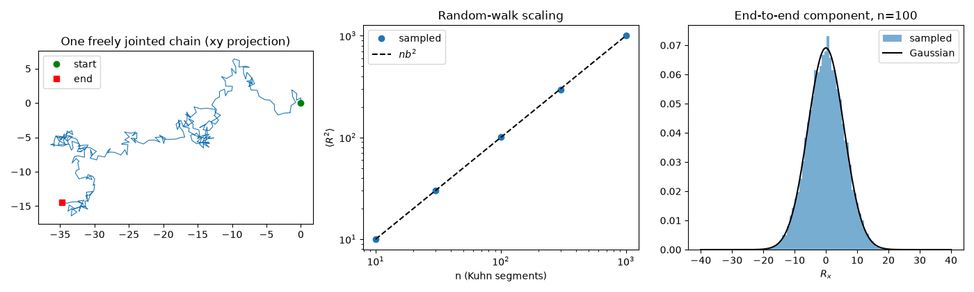
Kuhn (1934) modeled a flexible polymer as a random walk of \(n\) freely jointed segments of length \(b\). freely_jointed_chain() samples such conformations directly; averaging their squared end-to-end distance reproduces the exact result \(\langle R^2\rangle=nb^2\) (IdealChain), and the end-to-end vector’s components become Gaussian with variance \(nb^2/3\), as the central limit theorem predicts.

import matplotlib.pyplot as plt
import numpy as np

from chemistrykit.polymer.systems.chain_statistics import IdealChain, freely_jointed_chain

b = 1.0
ideal = IdealChain()
n_values = np.array([10, 30, 100, 300, 1000])

print("  n    <R^2> sampled   n b^2 (Kuhn)")
R2_sampled = []
for n in n_values:
    X = freely_jointed_chain(int(n), b, n_chains=4000, rng=int(n))
    R2 = np.sum(X[:, -1] ** 2, axis=-1).mean()
    R2_sampled.append(R2)
    print(f"{n:5d}   {R2:12.1f}   {ideal.mean_square_end_to_end(n, b):10.1f}")

 n    <R^2> sampled   n b^2 (Kuhn)
  10            9.9         10.0
  30           30.1         30.0
 100          100.3        100.0
 300          296.7        300.0
1000         1005.3       1000.0

The end-to-end x-component over many 100-segment chains is Gaussian with variance n b^2 / 3.

n = 100
X = freely_jointed_chain(n, b, n_chains=20000, rng=0)
Rx = X[:, -1, 0]
print(f"\nvar(R_x) = {Rx.var():.2f}  (Kuhn: n b^2 / 3 = {n * b**2 / 3:.2f})")

var(R_x) = 33.94  (Kuhn: n b^2 / 3 = 33.33)

fig, axes = plt.subplots(1, 3, figsize=(14, 4.2))
walk = freely_jointed_chain(300, b, rng=7)[0]
axes[0].plot(walk[:, 0], walk[:, 1], lw=0.8)
axes[0].plot(*walk[0, :2], "go", label="start")
axes[0].plot(*walk[-1, :2], "rs", label="end")
axes[0].set_aspect("equal")
axes[0].set_title("One freely jointed chain (xy projection)")
axes[0].legend()

axes[1].loglog(n_values, R2_sampled, "o", label="sampled")
axes[1].loglog(n_values, ideal.mean_square_end_to_end(n_values, b), "k--", label=r"$nb^2$")
axes[1].set_xlabel("n (Kuhn segments)")
axes[1].set_ylabel(r"$\langle R^2\rangle$")
axes[1].set_title("Random-walk scaling")
axes[1].legend()

grid = np.linspace(-40, 40, 300)
s2 = n * b**2 / 3
axes[2].hist(Rx, bins=60, density=True, alpha=0.6, label="sampled")
axes[2].plot(grid, np.exp(-(grid**2) / (2 * s2)) / np.sqrt(2 * np.pi * s2), "k", label="Gaussian")
axes[2].set_xlabel(r"$R_x$")
axes[2].set_title("End-to-end component, n=100")
axes[2].legend()
plt.tight_layout()
plt.show()