The Henderson-Hasselbalch equation and buffer design

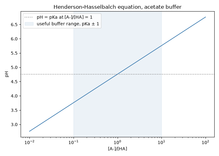
Hasselbalch’s logarithmic form of Henderson’s buffer relationship,

\[\mathrm{pH} = pK_a + \log_{10}\frac{[A^-]}{[HA]},\]

evaluated with henderson_hasselbalch_ph() and inverted by from_target_ph() to design an acetate buffer of fixed total concentration for any target pH. The equation is checked against the exact equilibrium pH of the same mixture.

import matplotlib.pyplot as plt
import numpy as np

from chemistrykit.solutions.systems.acid_base import Buffer, henderson_hasselbalch_ph

pKa = 4.76  # acetic acid
ratios = np.logspace(-2, 2, 200)
pH_hh = [henderson_hasselbalch_ph(pKa, base_conc=r, acid_conc=1.0) for r in ratios]

fig, ax = plt.subplots(figsize=(7, 5))
ax.semilogx(ratios, pH_hh, color="steelblue")
ax.axhline(pKa, color="gray", linestyle=":", label="pH = pKa at [A-]/[HA] = 1")
ax.axvspan(0.1, 10.0, color="steelblue", alpha=0.1, label="useful buffer range, pKa ± 1")
ax.set_xlabel("[A-]/[HA]")
ax.set_ylabel("pH")
ax.set_title("Henderson-Hasselbalch equation, acetate buffer")
ax.legend()
fig.tight_layout()

Designing a 0.20 M acetate buffer at pH 5.00, and plotting the required composition for every target pH:

buf = Buffer.from_target_ph(pKa=pKa, target_pH=5.0, total_conc=0.20)
print(f"Buffer: [HA] = {buf.acid_conc:.4f} M, [A-] = {buf.base_conc:.4f} M, pH = {buf.pH():.4f}")

pH_targets = np.linspace(pKa - 1.0, pKa + 1.0, 100)
base_fraction = [Buffer.from_target_ph(pKa=pKa, target_pH=pH, total_conc=0.20).base_conc / 0.20 for pH in pH_targets]

fig2, ax2 = plt.subplots(figsize=(7, 5))
ax2.plot(pH_targets, base_fraction, color="darkorange")
ax2.axvline(pKa, color="gray", linestyle=":", label="pH = pKa")
ax2.set_xlabel("target buffer pH")
ax2.set_ylabel("fraction as conjugate base, [A-]/C")
ax2.set_title("Buffer composition from Henderson-Hasselbalch")
ax2.legend()
fig2.tight_layout()

plt.show()

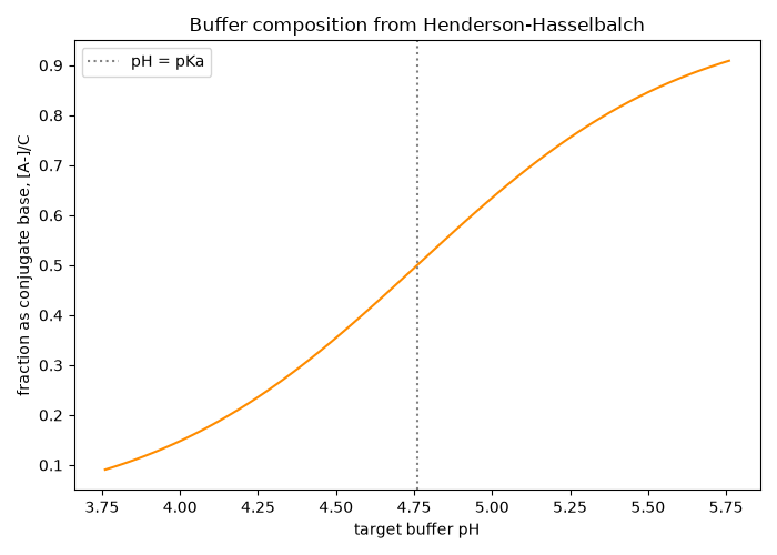
Buffer: [HA] = 0.0731 M, [A-] = 0.1269 M, pH = 5.0000