Bjerrum’s speciation diagrams for polyprotic acids

Niels Bjerrum’s 1914 monograph on acid-base titrations introduced diagrams showing what fraction of a polyprotic acid is present in each protonation state as a function of pH – today called Bjerrum plots or distribution diagrams. The fractions (polyprotic_fractions()) depend only on pH and the stepwise \(K_a\) values, and adjacent species are equally abundant exactly where \(\mathrm{pH} = pK_j\).

import matplotlib.pyplot as plt
import numpy as np

from chemistrykit.solutions.systems.acid_base import polyprotic_fractions

pH = np.linspace(0, 14, 500)

systems = {
    "carbonic acid": ([6.35, 10.33], ["H$_2$CO$_3$", "HCO$_3^-$", "CO$_3^{2-}$"]),
    "phosphoric acid": ([2.15, 7.20, 12.35], ["H$_3$PO$_4$", "H$_2$PO$_4^-$", "HPO$_4^{2-}$", "PO$_4^{3-}$"]),
}

fig, axes = plt.subplots(1, 2, figsize=(12, 4.5))
for ax, (name, (pKas, labels)) in zip(axes, systems.items()):
    alpha = polyprotic_fractions(pH, [10.0**-pK for pK in pKas])
    for row, label in zip(alpha, labels):
        ax.plot(pH, row, label=label)
    for pK in pKas:
        ax.axvline(pK, color="gray", linestyle=":", linewidth=0.8)
    ax.set_xlabel("pH")
    ax.set_ylabel(r"fraction $\alpha_j$")
    ax.set_title(f"Bjerrum plot: {name}")
    ax.legend(fontsize=8)
fig.tight_layout()

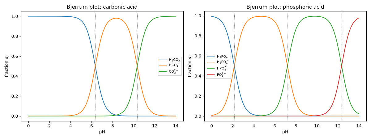
At blood pH 7.4, dissolved inorganic carbon is overwhelmingly bicarbonate – the basis of the bicarbonate blood buffer:

alpha_blood = polyprotic_fractions(7.4, [10**-6.35, 10**-10.33])[:, 0]
print("pH 7.4 carbonate speciation: " + ", ".join(f"{a:.4f}" for a in alpha_blood))

plt.show()

pH 7.4 carbonate speciation: 0.0817, 0.9172, 0.0011