Le Chatelier’s principle: the common-ion effect on AgCl solubility

Le Chatelier’s principle says an equilibrium disturbed by adding one of its participants shifts to consume it. Adding chloride to saturated AgCl drives \(\text{AgCl}(s) \rightleftharpoons \text{Ag}^+ + \text{Cl}^-\) back toward the solid, so AgCl’s molar solubility (molar_solubility_from_ksp()) drops sharply as increasing concentrations of a common ion (here, Cl- from added NaCl) are introduced – the direction Le Chatelier predicts, and the size quantified exactly by molar_solubility_with_common_ion().

import matplotlib.pyplot as plt
import numpy as np

from chemistrykit.solutions.systems.solubility import (
    molar_solubility_from_ksp,
    molar_solubility_with_common_ion,
)

Ksp_AgCl = 1.8e-10
s_pure = molar_solubility_from_ksp(Ksp_AgCl, cation_coeff=1, anion_coeff=1)
print(f"Molar solubility of AgCl in pure water: {s_pure:.3e} mol/L")

Cl_added = np.logspace(-4, -1, 60)
s_common = [molar_solubility_with_common_ion(Ksp_AgCl, 1, 1, C0, common_ion="anion") for C0 in Cl_added]

fig, ax = plt.subplots(figsize=(7, 5))
ax.loglog(Cl_added, s_common, color="steelblue", label="with added Cl-")
ax.axhline(s_pure, color="gray", linestyle=":", label="solubility in pure water")
ax.set_xlabel("[Cl-] added (mol/L)")
ax.set_ylabel("AgCl molar solubility (mol/L)")
ax.set_title("Common-ion suppression of AgCl solubility")
ax.legend()
fig.tight_layout()

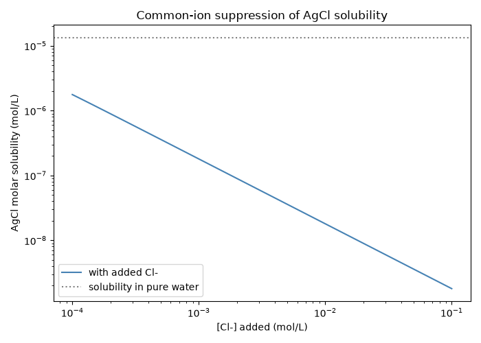
Molar solubility of AgCl in pure water: 1.342e-05 mol/L

At high added Cl-, the salt’s own contribution to [Cl-] becomes negligible, so s ~= Ksp/[Cl-] – a straight line on this log-log plot, which the numerical solver’s curve should approach:

s_approx = Ksp_AgCl / Cl_added
print(f"At [Cl-]=0.10 M: exact s = {s_common[-1]:.3e}, approximation Ksp/[Cl-] = {s_approx[-1]:.3e}")

plt.show()

At [Cl-]=0.10 M: exact s = 1.800e-09, approximation Ksp/[Cl-] = 1.800e-09