Nernst’s solubility product: Ksp for salts of any stoichiometry

Nernst showed that for a sparingly soluble salt \(M_pX_q\) in equilibrium with its saturated solution, the product of the ion concentrations, each raised to its stoichiometric coefficient, is a constant:

\[K_{sp} = [M]^p[X]^q = p^p q^q s^{p+q}.\]

ksp_from_molar_solubility() and its inverse molar_solubility_from_ksp() convert between the measured molar solubility \(s\) and \(K_{sp}\). Because the exponent \(p+q\) depends on stoichiometry, a smaller \(K_{sp}\) does not always mean a less soluble salt.

import matplotlib.pyplot as plt
import numpy as np

from chemistrykit.solutions.systems.solubility import ksp_from_molar_solubility, molar_solubility_from_ksp

salts = {
    "AgCl (1:1)": (1.8e-10, 1, 1),
    "CaF$_2$ (1:2)": (3.9e-11, 1, 2),
    "Ag$_2$CrO$_4$ (2:1)": (1.1e-12, 2, 1),
    "Ca$_3$(PO$_4$)$_2$ (3:2)": (2.1e-33, 3, 2),
}

Ksp_axis = np.logspace(-35, -5, 200)
fig, ax = plt.subplots(figsize=(7, 5))
for (name, (Ksp, p, q)), color in zip(salts.items(), ["steelblue", "darkorange", "seagreen", "purple"]):
    ax.loglog(Ksp_axis, molar_solubility_from_ksp(Ksp_axis, p, q), color=color, alpha=0.5)
    s = molar_solubility_from_ksp(Ksp, p, q)
    ax.plot(Ksp, s, "o", color=color, label=f"{name}: s = {s:.1e} M")
ax.set_xlabel("solubility product $K_{sp}$")
ax.set_ylabel("molar solubility s (mol/L)")
ax.set_title(r"Solubility product: $s = (K_{sp}/p^pq^q)^{1/(p+q)}$")
ax.legend(fontsize=8)
fig.tight_layout()

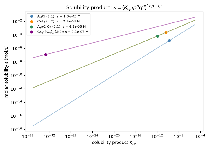
Ag2CrO4 has a smaller Ksp than AgCl yet is more soluble – the comparison only works between salts of the same stoichiometry. The round trip s -> Ksp -> s is exact:

for name, (Ksp, p, q) in salts.items():
    s = molar_solubility_from_ksp(Ksp, p, q)
    plain = name.replace("$", "").replace("_", "")
    print(f"{plain:22s}: Ksp = {Ksp:.1e}, s = {s:.3e} M, Ksp from s = {ksp_from_molar_solubility(s, p, q):.2e}")

plt.show()

AgCl (1:1)            : Ksp = 1.8e-10, s = 1.342e-05 M, Ksp from s = 1.80e-10
CaF2 (1:2)            : Ksp = 3.9e-11, s = 2.136e-04 M, Ksp from s = 3.90e-11
Ag2CrO4 (2:1)         : Ksp = 1.1e-12, s = 6.503e-05 M, Ksp from s = 1.10e-12
Ca3(PO4)2 (3:2)       : Ksp = 2.1e-33, s = 1.142e-07 M, Ksp from s = 2.10e-33