Fraunhofer’s dark lines: sharp absorption lines at fixed wavelengths in the solar spectrum

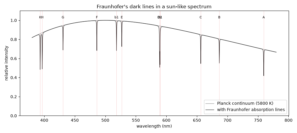
Fraunhofer (1814) found that sunlight is not a smooth rainbow but a continuum crossed by hundreds of sharp dark lines at fixed, reproducible wavelengths, and he labelled the strongest ones A to K. This example builds a sun-like continuum from Planck’s law at 5800 K, removes light at the tabulated positions of Fraunhofer’s lettered lines using narrow Lorentzian absorption profiles, and marks each letter above its line.

import matplotlib.pyplot as plt
import numpy as np
import scipy.constants as sc

from chemistrykit.spectro.core.base_system import Spectrum

# Fraunhofer's lettered lines (air wavelengths in nm) and their modern
# assignments -- the originals were only positions; the atoms came later.
fraunhofer_lines = {
    "A (O2)": 759.4,
    "B (O2)": 686.7,
    "C (H-alpha)": 656.3,
    "D1 (Na)": 589.6,
    "D2 (Na)": 589.0,
    "E (Fe)": 527.0,
    "b1 (Mg)": 518.4,
    "F (H-beta)": 486.1,
    "G (Fe/CH)": 430.8,
    "H (Ca+)": 396.8,
    "K (Ca+)": 393.4,
}
depths = np.array([0.8, 0.6, 0.7, 0.8, 0.9, 0.5, 0.6, 0.6, 0.5, 0.9, 0.9])
lines = Spectrum(positions=list(fraunhofer_lines.values()), intensities=depths, labels=list(fraunhofer_lines))

wavelength_nm = np.linspace(380.0, 780.0, 8000)
lam = wavelength_nm * 1e-9
temperature = 5800.0
planck = (2.0 * sc.h * sc.c**2 / lam**5) / np.expm1(sc.h * sc.c / (lam * sc.k * temperature))
continuum = planck / planck.max()

# Each dark line removes a fraction of the local continuum: an optical
# depth given by a narrow Lorentzian profile centred on the line.
optical_depth = lines.broaden(wavelength_nm, shape="lorentzian", fwhm=0.4) * 0.4
observed = continuum * np.exp(-optical_depth)

for label, position in zip(lines.labels, lines.positions, strict=True):
    i = np.argmin(np.abs(wavelength_nm - position))
    print(f"{label:>12s} at {position:6.1f} nm: transmitted fraction {observed[i] / continuum[i]:.2f}")

     A (O2) at  759.4 nm: transmitted fraction 0.60
     B (O2) at  686.7 nm: transmitted fraction 0.68
C (H-alpha) at  656.3 nm: transmitted fraction 0.64
    D1 (Na) at  589.6 nm: transmitted fraction 0.57
    D2 (Na) at  589.0 nm: transmitted fraction 0.54
     E (Fe) at  527.0 nm: transmitted fraction 0.73
    b1 (Mg) at  518.4 nm: transmitted fraction 0.68
 F (H-beta) at  486.1 nm: transmitted fraction 0.68
  G (Fe/CH) at  430.8 nm: transmitted fraction 0.73
    H (Ca+) at  396.8 nm: transmitted fraction 0.56
    K (Ca+) at  393.4 nm: transmitted fraction 0.56

The dark lines stand out sharply against the smooth continuum – the pattern of fixed line positions Fraunhofer showed is reproducible, and which later became a fingerprint of the Sun’s chemical composition.

fig, ax = plt.subplots(figsize=(10, 4.5))
ax.plot(wavelength_nm, continuum, color="0.6", lw=1, label="Planck continuum (5800 K)")
ax.plot(wavelength_nm, observed, color="black", lw=0.8, label="with Fraunhofer absorption lines")
for label, position in zip(lines.labels, lines.positions, strict=True):
    ax.annotate(label.split()[0], (position, 1.02), ha="center", fontsize=8)
    ax.axvline(position, color="tab:red", lw=0.4, alpha=0.4)
ax.set_xlabel("wavelength (nm)")
ax.set_ylabel("relative intensity")
ax.set_ylim(0.0, 1.1)
ax.set_title("Fraunhofer's dark lines in a sun-like spectrum")
ax.legend(loc="lower right")
fig.tight_layout()
plt.show()