The hydrogen spectrum: Balmer’s formula, the Rydberg series, and Bohr’s energy levels

Balmer (1885) fitted the four visible hydrogen lines with \(\lambda=B\,n^2/(n^2-4)\). Rydberg (1890) rewrote this in wavenumbers as \(\tilde\nu=R(1/n_1^2-1/n_2^2)\), and Bohr (1913) derived it from quantized electron energies \(E_n=-hcR/n^2\). This example computes the Lyman, Balmer, and Paschen series with rydberg_wavenumber(), checks the result against Balmer’s original formula, and shows each series bunching toward its series limit.

import matplotlib.pyplot as plt
import numpy as np
import scipy.constants as sc

from chemistrykit.spectro.systems.atomic import rydberg_wavenumber

n_upper = np.arange(3, 8)
balmer_nu = rydberg_wavenumber(2, n_upper, nuclear_mass=sc.m_p)
balmer_nm = 1e7 / balmer_nu

# Balmer's constant B = 4 / R_H (his fitted value, in air, was 364.56 nm).
B = 4.0 / (sc.Rydberg / 100.0 / (1.0 + sc.m_e / sc.m_p)) * 1e7
print(f"Balmer's constant B = 4/R_H = {B:.2f} nm (vacuum)")
for n, lam in zip(n_upper, balmer_nm, strict=True):
    print(f"  n={n} -> 2: Rydberg {lam:7.2f} nm, Balmer formula {B * n**2 / (n**2 - 4):7.2f} nm")

Balmer's constant B = 4/R_H = 364.71 nm (vacuum)
  n=3 -> 2: Rydberg  656.47 nm, Balmer formula  656.47 nm
  n=4 -> 2: Rydberg  486.27 nm, Balmer formula  486.27 nm
  n=5 -> 2: Rydberg  434.17 nm, Balmer formula  434.17 nm
  n=6 -> 2: Rydberg  410.29 nm, Balmer formula  410.29 nm
  n=7 -> 2: Rydberg  397.12 nm, Balmer formula  397.12 nm

Each series converges on a limit (\(n_2\to\infty\)) equal to \(R_H/n_1^2\), the energy needed to ionize an atom that starts in level \(n_1\). The first three series fall in the ultraviolet, visible, and infrared.

series = {"Lyman (n1=1)": 1, "Balmer (n1=2)": 2, "Paschen (n1=3)": 3}
fig, axes = plt.subplots(3, 1, figsize=(10, 7))
for ax, (name, n1) in zip(axes, series.items(), strict=True):
    n2 = np.arange(n1 + 1, n1 + 25)
    nu = rydberg_wavenumber(n1, n2, nuclear_mass=sc.m_p)
    limit = rydberg_wavenumber(n1, 10**9, nuclear_mass=sc.m_p)
    ax.vlines(nu, 0.0, 1.0 / (n2 - n1) ** 1.5, color="tab:blue")
    ax.axvline(limit, color="tab:red", ls="--", lw=1, label=f"series limit {limit:.0f} cm$^{{-1}}$")
    ax.set_title(name)
    ax.set_ylabel("rel. intensity")
    ax.legend(loc="upper left")
    print(f"{name}: first line {1e7 / nu[0]:.1f} nm, limit {1e7 / limit:.1f} nm")
axes[-1].set_xlabel(r"wavenumber (cm$^{-1}$)")
fig.suptitle("Hydrogen line series from the Rydberg formula")
fig.tight_layout()

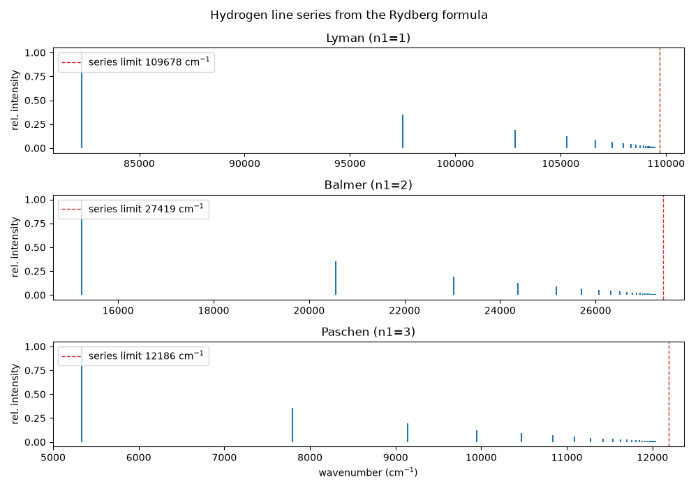
Lyman (n1=1): first line 121.6 nm, limit 91.2 nm
Balmer (n1=2): first line 656.5 nm, limit 364.7 nm
Paschen (n1=3): first line 1875.6 nm, limit 820.6 nm

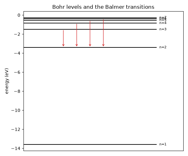
Bohr’s energy levels explain the series: every line is a jump between two levels \(E_n=-hcR_H/n^2\).

fig2, ax2 = plt.subplots(figsize=(6, 5))
r_h_ev = sc.h * sc.c * sc.Rydberg / (1.0 + sc.m_e / sc.m_p) / sc.e
for n in range(1, 8):
    ax2.hlines(-r_h_ev / n**2, 0.0, 1.0, color="black")
    ax2.annotate(f"n={n}", (1.02, -r_h_ev / n**2), va="center", fontsize=8)
for i, n in enumerate(range(3, 7)):
    ax2.annotate("", xy=(0.3 + 0.1 * i, -r_h_ev / 4), xytext=(0.3 + 0.1 * i, -r_h_ev / n**2), arrowprops={"arrowstyle": "->", "color": "tab:red"})
ax2.set_xlim(0.0, 1.2)
ax2.set_xticks([])
ax2.set_ylabel("energy (eV)")
ax2.set_title("Bohr levels and the Balmer transitions")
fig2.tight_layout()
plt.show()