Second-order NMR: from AX to AB, and the ABX system

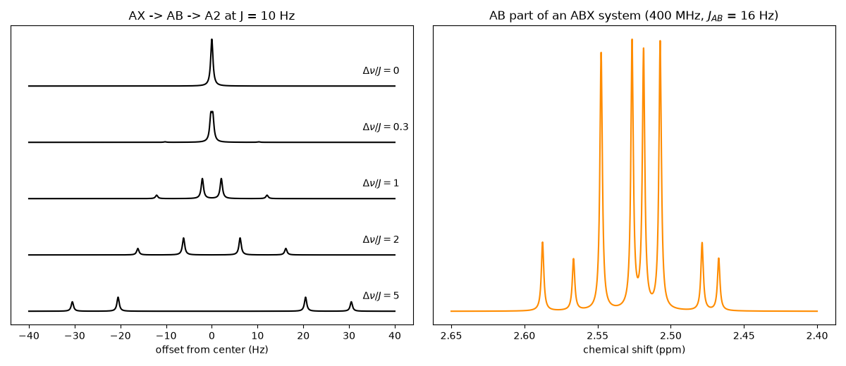
First-order rules (doublets of equal lines, spaced by \(J\), centered on each shift) hold only while \(\Delta\nu \gg J\). As the two shifts approach each other the doublets lean toward one another: the inner lines grow and the outer ones shrink, the “roof effect”. At \(\Delta\nu=0\) the two nuclei become equivalent and a single line remains. second_order_spectrum() diagonalizes the full spin Hamiltonian, and ab_quartet() gives the closed-form AB result it must agree with. The right panel is an ABX system (abx_spectrum()), the case Bernstein, Pople and Schneider analyzed: a strongly coupled CH2 pair (AB) next to a distant CH (X). Its AB part is no longer two simple doublets of doublets.

import matplotlib.pyplot as plt
import numpy as np

from chemistrykit.spectro import ab_quartet, abx_spectrum, second_order_spectrum

nu0 = 400.0  # MHz
J = 10.0  # Hz
ratios = [5.0, 2.0, 1.0, 0.3, 0.0]  # delta_nu / J

fig, axes = plt.subplots(1, 2, figsize=(12, 5.2))
x = np.linspace(-40, 40, 4000)
for k, ratio in enumerate(ratios):
    delta_ppm = ratio * J / nu0
    s = second_order_spectrum([2.0 - delta_ppm / 2, 2.0 + delta_ppm / 2], [[0, J], [J, 0]], nu0)
    hz = (s.positions - 2.0) * nu0
    line = sum(a * 0.3**2 / ((x - p) ** 2 + 0.3**2) for p, a in zip(hz, s.intensities, strict=True))
    axes[0].plot(x, line / 4 + 1.2 * k, color="black")
    axes[0].text(33, 1.2 * k + 0.25, rf"$\Delta\nu/J={ratio:g}$")
axes[0].set_xlabel("offset from center (Hz)")
axes[0].set_yticks([])
axes[0].set_title("AX -> AB -> A2 at J = 10 Hz")

abx = abx_spectrum([2.50, 2.55, 4.20], j_ab_hz=16.0, j_ax_hz=4.0, j_bx_hz=9.0, spectrometer_frequency_mhz=nu0)
ppm = np.linspace(2.40, 2.65, 3000)
ab_part = abx.positions < 3.0
line = sum(a * 0.001**2 / ((ppm - p) ** 2 + 0.001**2) for p, a in zip(abx.positions[ab_part], abx.intensities[ab_part], strict=True))
axes[1].plot(ppm, line, color="darkorange")
axes[1].invert_xaxis()
axes[1].set_xlabel("chemical shift (ppm)")
axes[1].set_yticks([])
axes[1].set_title(r"AB part of an ABX system (400 MHz, $J_{AB}$ = 16 Hz)")
fig.tight_layout()

The exact diagonalization reproduces the closed-form AB quartet:

s = second_order_spectrum([2.00, 2.02], [[0, J], [J, 0]], nu0)
q = ab_quartet(2.00, 2.02, J, nu0)
print("exact  :", np.round(s.intensities, 4))
print("formula:", np.round(q.intensities, 4))
print(f"ABX: {int(ab_part.sum())} AB lines, {int((~ab_part).sum())} X lines, total intensity {abx.intensities.sum():.1f}")

plt.show()

exact  : [0.2191 1.7809 1.7809 0.2191]
formula: [0.2191 1.7809 1.7809 0.2191]
ABX: 8 AB lines, 6 X lines, total intensity 12.0