Dennison’s quantized rigid rotor: HCl rotational lines spaced by 2B, with Boltzmann intensities

Dennison (1926) gave the quantum-mechanical rotational energy levels \(E_J=\hbar^2J(J+1)/(2I)\). With the \(\Delta J=+1\) selection rule, these levels produce absorption lines at \(2B(J+1)\), which are evenly spaced by \(2B\). This example builds an HCl-like rigid rotor from chemistrykit.quantum, prints its level energies and line positions, checks the constant \(2B\) spacing, and adds the Boltzmann-population intensity pattern seen in a real far-infrared or microwave spectrum.

import matplotlib.pyplot as plt
import numpy as np
import scipy.constants as sc

from chemistrykit.quantum.systems.rigid_rotor import RigidRotor
from chemistrykit.spectro.systems.rotational import energy_to_wavenumber, rotational_line_wavenumbers, rotational_spectrum
from chemistrykit.spectro.visualizers.spectro_plots import plot_broadened_spectrum, plot_stick_spectrum

rotor_hcl = RigidRotor.from_diatomic(mass1=1.008 * sc.atomic_mass, mass2=34.97 * sc.atomic_mass, bond_length=127.5e-12)

levels = np.array([energy_to_wavenumber(rotor_hcl.energy(J)) for J in range(6)])
print(f"Rotational levels E_J/hc (cm^-1), J=0..5: {np.round(levels, 2)}")
B = levels[1] / 2.0  # E_1 = 2B
print(f"Rotational constant B = {B:.3f} cm^-1; E_J / B = {np.round(levels / B, 3)} = J(J+1)")

Rotational levels E_J/hc (cm^-1), J=0..5: [  0.    21.17  63.51 127.01 211.68 317.53]
Rotational constant B = 10.584 cm^-1; E_J / B = [ 0.  2.  6. 12. 20. 30.] = J(J+1)

Transitions \(J\to J+1\) fall at \(2B(J+1)\), which gives an evenly spaced line pattern, even though the levels themselves are not evenly spaced:

lines_hcl = rotational_line_wavenumbers(rotor_hcl, J_max=8)
print(f"HCl lines (cm^-1): {np.round(lines_hcl, 2)}")
print(f"Line spacings (cm^-1): {np.round(np.diff(lines_hcl), 3)}  (2B = {2 * B:.3f})")

HCl lines (cm^-1): [ 21.17  42.34  63.51  84.67 105.84 127.01 148.18 169.35 190.52]
Line spacings (cm^-1): [21.168 21.168 21.168 21.168 21.168 21.168 21.168 21.168]  (2B = 21.168)

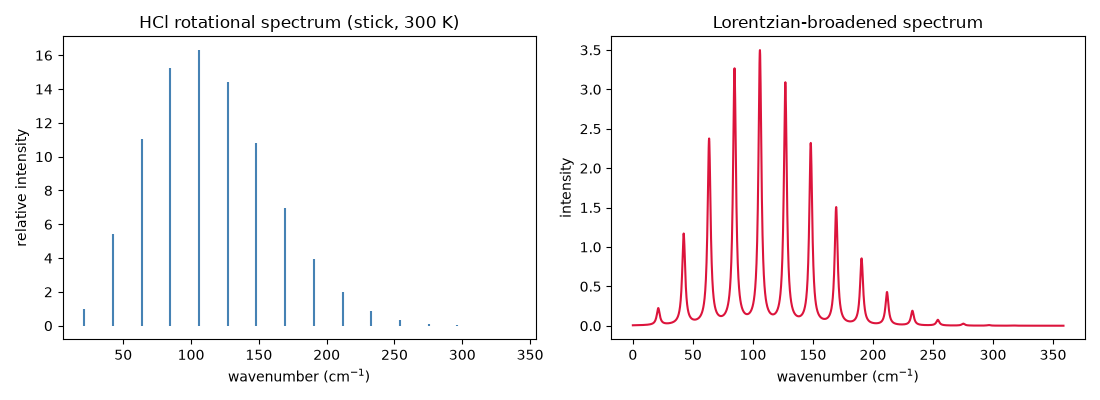
The full spectrum, with relative intensities from the Boltzmann population and \((2J+1)\) degeneracy of each initial J level. The strongest line comes from the most populated level, not from J=0:

spectrum = rotational_spectrum(rotor_hcl, J_max=15, temperature=300.0)
fig, (ax1, ax2) = plt.subplots(1, 2, figsize=(11, 4))
plot_stick_spectrum(spectrum, ax=ax1, color="steelblue")
ax1.set_xlabel(r"wavenumber (cm$^{-1}$)")
ax1.set_title("HCl rotational spectrum (stick, 300 K)")

x = np.linspace(0, spectrum.positions[-1] + 20.0, 2000)
plot_broadened_spectrum(spectrum, x, ax=ax2, shape="lorentzian", fwhm=3.0, color="crimson")
ax2.set_xlabel(r"wavenumber (cm$^{-1}$)")
ax2.set_title("Lorentzian-broadened spectrum")

fig.tight_layout()
plt.show()