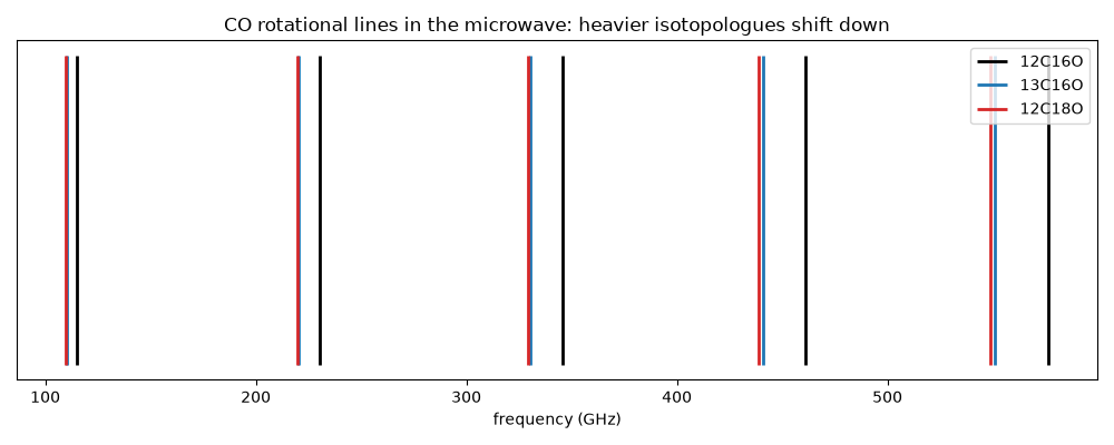
Microwave spectroscopy and the isotope shift: CO isotopologues’ J=1-0 lines in GHz

Rotational lines of light molecules lie in the microwave region, which became routinely accessible after Cleeton and Williams (1934) and postwar microwave spectroscopy by Townes and others. Microwave frequencies can be measured very precisely, so isotope shifts are easy to see. Isotopic substitution leaves the bond length unchanged but changes the reduced mass, so every line of the heavier isotopologue moves down by \(\mu_a/\mu_b\), the ratio isotope_shift_ratio() predicts. This example computes the \(J=1\leftarrow0\) lines of \(^{12}\mathrm{C}^{16}\mathrm{O}\), \(^{13}\mathrm{C}^{16}\mathrm{O}\) and \(^{12}\mathrm{C}^{18}\mathrm{O}\) in GHz and compares them with the measured values (115.271, 110.201 and 109.782 GHz).

import matplotlib.pyplot as plt
import numpy as np
import scipy.constants as sc

from chemistrykit.quantum.systems.rigid_rotor import RigidRotor
from chemistrykit.spectro.systems.rotational import isotope_shift_ratio, rotational_line_wavenumbers

u = sc.atomic_mass
r_co = 113.09e-12  # m, ground-state (r_0) C-O bond length, shared by all isotopologues
isotopologues = {
    "12C16O": (12.000 * u, 15.995 * u, 115.271),
    "13C16O": (13.003 * u, 15.995 * u, 110.201),
    "12C18O": (12.000 * u, 17.999 * u, 109.782),
}

frequencies_ghz = {}
for name, (m_c, m_o, measured) in isotopologues.items():
    rotor = RigidRotor.from_diatomic(mass1=m_c, mass2=m_o, bond_length=r_co)
    nu_cm = rotational_line_wavenumbers(rotor, J_max=4)
    frequencies_ghz[name] = nu_cm * 100.0 * sc.c / 1e9
    print(f"{name}: J=1<-0 predicted {frequencies_ghz[name][0]:.3f} GHz, measured {measured:.3f} GHz")

12C16O: J=1<-0 predicted 115.269 GHz, measured 115.271 GHz
13C16O: J=1<-0 predicted 110.189 GHz, measured 110.201 GHz
12C18O: J=1<-0 predicted 109.768 GHz, measured 109.782 GHz

The frequency ratio for any isotopologue pair is the inverse ratio of their reduced masses. It is the same for every line, and it matches isotope_shift_ratio:

ratio_13c = isotope_shift_ratio(mass1a=12.000 * u, mass2=15.995 * u, mass1b=13.003 * u)
observed_ratio = frequencies_ghz["13C16O"] / frequencies_ghz["12C16O"]
print(f"isotope_shift_ratio(12C->13C) = {ratio_13c:.5f}; line-by-line ratios {np.round(observed_ratio, 5)}")
print(f"Measured ratio 110.201/115.271 = {110.201 / 115.271:.5f}")

isotope_shift_ratio(12C->13C) = 0.95593; line-by-line ratios [0.95593 0.95593 0.95593 0.95593 0.95593]
Measured ratio 110.201/115.271 = 0.95602

fig, ax = plt.subplots(figsize=(10, 4))
colors = {"12C16O": "black", "13C16O": "tab:blue", "12C18O": "tab:red"}
for name, freqs in frequencies_ghz.items():
    ax.vlines(freqs, 0.0, 1.0, color=colors[name], lw=2, label=name)
ax.set_xlabel("frequency (GHz)")
ax.set_yticks([])
ax.set_title("CO rotational lines in the microwave: heavier isotopologues shift down")
ax.legend()
fig.tight_layout()
plt.show()