Harmonic vs. Morse IR band positions, and recovering anharmonicity from overtones

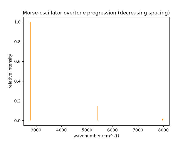
Predicts HCl’s fundamental IR absorption from a harmonic oscillator, compares it against the exact (anharmonic) Morse-potential fundamental and first overtone, then inverts the observed \(0\to1\)/\(0\to2\) band positions to recover the spectroscopic constants \(\omega_e\)/\(\omega_ex_e\) – exactly the way real anharmonicity constants are measured from an observed overtone spectrum.

import matplotlib.pyplot as plt
import scipy.constants as sc

from chemistrykit.quantum.systems.harmonic_oscillator import MorseOscillator
from chemistrykit.spectro.core.base_system import Spectrum
from chemistrykit.spectro.systems.vibrational import anharmonicity_from_overtones, harmonic_fundamental_wavenumber, morse_transition_wavenumbers
from chemistrykit.spectro.visualizers.spectro_plots import plot_stick_spectrum

mu = (1.008 * 34.97) / (1.008 + 34.97) * sc.atomic_mass  # HCl-like reduced mass
k = 480.0  # N/m
De = 7.24e-19  # J, HCl-like dissociation energy

harmonic_nu = harmonic_fundamental_wavenumber(force_constant=k, reduced_mass=mu)
print(f"Harmonic fundamental: {harmonic_nu:.1f} cm^-1")

morse = MorseOscillator(mass=mu, force_constant=k, dissociation_energy=De)
nu01, nu02, nu03 = morse_transition_wavenumbers(morse, v_max=3)
print(f"Morse fundamental (0->1): {nu01:.1f} cm^-1")
print(f"Morse first overtone (0->2): {nu02:.1f} cm^-1 (would be {2 * nu01:.1f} cm^-1 if purely harmonic)")

Harmonic fundamental: 2883.6 cm^-1
Morse fundamental (0->1): 2769.5 cm^-1
Morse first overtone (0->2): 5425.0 cm^-1 (would be 5539.1 cm^-1 if purely harmonic)

Recovering the spectroscopic constants from just these two observed band positions – exactly, no fitting – and confirming they predict the (unused, held-out) third overtone correctly:

omega_e, omega_e_xe = anharmonicity_from_overtones(nu01, nu02)
print(f"Recovered omega_e = {omega_e:.1f} cm^-1, omega_e*xe = {omega_e_xe:.2f} cm^-1")

predicted_nu03 = 3.0 * omega_e - 12.0 * omega_e_xe
print(f"Predicted 0->3 overtone: {predicted_nu03:.1f} cm^-1 (actual: {nu03:.1f} cm^-1)")

Recovered omega_e = 2883.6 cm^-1, omega_e*xe = 57.04 cm^-1
Predicted 0->3 overtone: 7966.4 cm^-1 (actual: 7966.4 cm^-1)

spectrum = Spectrum(positions=[nu01, nu02, nu03], intensities=[1.0, 0.15, 0.02], labels=["0->1", "0->2", "0->3"])
ax = plot_stick_spectrum(spectrum, color="darkorange")
ax.set_xlabel("wavenumber (cm^-1)")
ax.set_title("Morse-oscillator overtone progression (decreasing spacing)")
plt.show()