Wilson’s GF-matrix method: CO2 and H2O normal-mode frequencies from the G and F matrices

This example uses Wilson’s GF-matrix method to calculate normal modes for a linear triatomic (CO2) and a bent one (H2O) with TriatomicNormalModes. The molecule’s geometry and masses give the kinetic-energy matrix \(G=BM^{-1}B^T\), where \(B\) is the Wilson B-matrix. A diagonal valence force field gives the potential-energy matrix \(F\). Solving the eigenvalue problem \(GFL=L\Lambda\), with \(\lambda_k=(2\pi c\tilde\nu_k)^2\), gives the normal-mode wavenumbers. Changing only the bend entry of \(F\) shifts the bend frequency, while the stretches barely move.

import matplotlib.pyplot as plt
import scipy.constants as sc

from chemistrykit.spectro.systems.vibrational import TriatomicNormalModes

co2 = TriatomicNormalModes.linear(
    mass_terminal=15.999 * sc.atomic_mass,
    mass_central=12.011 * sc.atomic_mass,
    bond_length=116.3e-12,
    k_r=1600.0,
    k_theta=0.85e-18,
)
co2_result = co2.solve()
print("CO2 (linear) normal-mode wavenumbers (cm^-1):")
print(f"  bend (doubly degenerate): {co2_result.wavenumbers[0]:.1f}  (real: 667)")
print(f"  symmetric stretch (IR-inactive): {co2_result.wavenumbers[1]:.1f}  (real: 1388)")
print(f"  antisymmetric stretch: {co2_result.wavenumbers[2]:.1f}  (real: 2349)")

CO2 (linear) normal-mode wavenumbers (cm^-1):
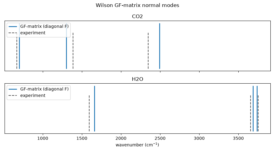
  bend (doubly degenerate): 699.0  (real: 667)
  symmetric stretch (IR-inactive): 1302.8  (real: 1388)
  antisymmetric stretch: 2493.8  (real: 2349)

water = TriatomicNormalModes.bent(
    mass_terminal=1.008 * sc.atomic_mass,
    mass_central=15.999 * sc.atomic_mass,
    bond_length=95.8e-12,
    bond_angle_degrees=104.5,
    k_r=770.0,
    k_theta=0.7e-18,
)
water_result = water.solve()
print("\nH2O (bent) normal-mode wavenumbers (cm^-1):")
print(f"  bend: {water_result.wavenumbers[0]:.1f}  (real: 1595)")
print(f"  symmetric stretch: {water_result.wavenumbers[1]:.1f}  (real: 3657)")
print(f"  antisymmetric stretch: {water_result.wavenumbers[2]:.1f}  (real: 3756)")

H2O (bent) normal-mode wavenumbers (cm^-1):
  bend: 1661.2  (real: 1595)
  symmetric stretch: 3686.3  (real: 3657)
  antisymmetric stretch: 3739.9  (real: 3756)

These come from a simple diagonal valence force field (no stretch-stretch or stretch-bend interaction constants) with literature-typical, but not precisely fitted, force constants – so they land in the right ballpark and reproduce the correct qualitative ordering (bend well below both stretches) without matching experiment to spectroscopic precision. Stiffening the bend force constant raises only the bend frequency, as expected for a diagonal force field:

soft_bend = TriatomicNormalModes.bent(
    mass_terminal=1.008 * sc.atomic_mass,
    mass_central=15.999 * sc.atomic_mass,
    bond_length=95.8e-12,
    bond_angle_degrees=104.5,
    k_r=770.0,
    k_theta=0.3e-18,
).solve()
stiff_bend = TriatomicNormalModes.bent(
    mass_terminal=1.008 * sc.atomic_mass,
    mass_central=15.999 * sc.atomic_mass,
    bond_length=95.8e-12,
    bond_angle_degrees=104.5,
    k_r=770.0,
    k_theta=1.2e-18,
).solve()
print(f"\nBend wavenumber with soft k_theta: {soft_bend.wavenumbers[0]:.1f} cm^-1")
print(f"Bend wavenumber with stiff k_theta: {stiff_bend.wavenumbers[0]:.1f} cm^-1")
print(f"Stretch wavenumbers unchanged: {soft_bend.wavenumbers[1:]} vs {stiff_bend.wavenumbers[1:]}")

Bend wavenumber with soft k_theta: 1087.8 cm^-1
Bend wavenumber with stiff k_theta: 2174.0 cm^-1
Stretch wavenumbers unchanged: [3685.35491056 3739.86728349] vs [3688.02836763 3739.86728349]

Computed GF-matrix wavenumbers (solid) next to the experimental fundamentals (dashed) for both molecules:

fig, axes = plt.subplots(2, 1, figsize=(9, 5), sharex=True)
for ax, name, computed, measured in (
    (axes[0], "CO2", co2_result.wavenumbers, [667.0, 1388.0, 2349.0]),
    (axes[1], "H2O", water_result.wavenumbers, [1595.0, 3657.0, 3756.0]),
):
    ax.vlines(computed, 0.0, 1.0, color="tab:blue", lw=2, label="GF-matrix (diagonal F)")
    ax.vlines(measured, 0.0, 0.8, color="0.3", ls="--", label="experiment")
    ax.set_yticks([])
    ax.set_title(name)
    ax.legend(loc="upper left")
axes[1].set_xlabel(r"wavenumber (cm$^{-1}$)")
fig.suptitle("Wilson GF-matrix normal modes")
fig.tight_layout()
plt.show()