Boltzmann’s S = k ln W by counting lattice arrangements

Boltzmann’s 1877 insight, written by Planck as \(S=k_B\ln W\): entropy counts the microscopic arrangements W compatible with a macroscopic state. For N indistinguishable molecules on M lattice sites, \(W=\binom{M}{N}\), and canonical_entropy() evaluates \(k_B\ln W\) exactly via ln_binomial(). The entropy is largest at half filling, where the number of arrangements peaks, and per site it converges to the Stirling-approximation mixing entropy \(-k_B[\theta\ln\theta+(1-\theta)\ln(1-\theta)]\) as M grows.

import math

import matplotlib.pyplot as plt
import numpy as np

from chemistrykit.constants import K_B
from chemistrykit.statmech import LatticeGasAdsorption

For a tiny lattice, W can be counted by hand and matches exp(S/k_B):

M_small = 6
for N in range(M_small + 1):
    W = math.comb(M_small, N)
    S = LatticeGasAdsorption.canonical_entropy(N, M_small)
    print(f"N = {N}: W = {W:2d}, exp(S/k_B) = {np.exp(S / K_B):.4f}")

N = 0: W =  1, exp(S/k_B) = 1.0000
N = 1: W =  6, exp(S/k_B) = 6.0000
N = 2: W = 15, exp(S/k_B) = 15.0000
N = 3: W = 20, exp(S/k_B) = 20.0000
N = 4: W = 15, exp(S/k_B) = 15.0000
N = 5: W =  6, exp(S/k_B) = 6.0000
N = 6: W =  1, exp(S/k_B) = 1.0000

For larger lattices, S/(M k_B) approaches the Stirling limit:

theta = np.linspace(0.001, 0.999, 400)
stirling = -(theta * np.log(theta) + (1.0 - theta) * np.log(1.0 - theta))

fig, axes = plt.subplots(1, 2, figsize=(11, 4.5))
for M, color in [(10, "crimson"), (50, "darkorange"), (1000, "steelblue")]:
    N_values = np.arange(0, M + 1)
    S = np.array([LatticeGasAdsorption.canonical_entropy(N, M) for N in N_values])
    axes[0].plot(N_values / M, S / (M * K_B), marker="o" if M <= 10 else None, color=color, label=f"exact, M = {M}")
axes[0].plot(theta, stirling, color="black", linestyle="--", label="Stirling limit")
axes[0].axvline(0.5, color="gray", linestyle=":", linewidth=0.8)
axes[0].set_xlabel(r"fractional filling $\theta = N/M$")
axes[0].set_ylabel(r"$S / (M k_B) = \ln W / M$")
axes[0].set_title(r"$S = k_B \ln W$ is largest at half filling")
axes[0].legend()

M = 100
N_values = np.arange(0, M + 1)
lnW = np.array([LatticeGasAdsorption.canonical_entropy(N, M) for N in N_values]) / K_B
axes[1].semilogy(N_values, np.exp(lnW), color="steelblue")
axes[1].set_xlabel("number of molecules N")
axes[1].set_ylabel("number of arrangements W")
axes[1].set_title(f"Microstate count on M = {M} sites")
fig.tight_layout()

plt.show()

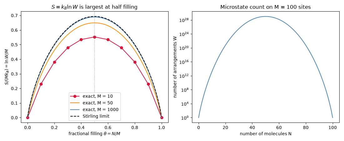
The half-filled lattice of 100 sites has about 1e29 arrangements, while a completely full or empty lattice has exactly one (S = 0): the overwhelming statistical weight of “disordered” states is what the second law expresses.