Einstein’s quantum theory of the vibrational heat capacity

Einstein (1907) treated each vibration as a quantum oscillator of frequency \(\nu\), so its heat capacity depends on \(\Theta_{\text{vib}}/T\) with \(\Theta_{\text{vib}}=h\nu/k_B\). VibrationalPartitionFunctionHarmonic’s heat capacity is this formula: it vanishes as \(T\to0\) (the vibration is “frozen out”) and approaches the classical equipartition value \(k_B\) per mode only once \(T\) is comparable to \(\Theta_{\text{vib}}\). The second plot shows why a stiff mode (like Einstein’s diamond) stays frozen out at temperatures where a soft mode already behaves classically.

import matplotlib.pyplot as plt
import numpy as np
import scipy.constants as sc

from chemistrykit.statmech import VibrationalPartitionFunctionHarmonic
from chemistrykit.statmech.visualizers.statmech_plots import plot_heat_capacity_vs_temperature

K_B = sc.k

hcl_mode = VibrationalPartitionFunctionHarmonic.from_wavenumber(2886.0)  # HCl fundamental, cm^-1
print(f"HCl vibrational temperature: {hcl_mode.vibrational_temperature:.1f} K")

T = np.linspace(50.0, 6000.0, 300)

fig, axes = plt.subplots(1, 2, figsize=(11, 4.5))
plot_heat_capacity_vs_temperature(hcl_mode, T, ax=axes[0], color="steelblue")
axes[0].axhline(K_B, color="gray", linestyle=":", linewidth=0.8, label="classical limit (k_B)")
axes[0].axvline(hcl_mode.vibrational_temperature, color="crimson", linestyle=":", linewidth=0.8, label="vibrational temperature")
axes[0].set_title("Einstein heat capacity of one mode (HCl-like)")
axes[0].legend()

# Plotted against reduced temperature T / Theta_vib, every Einstein mode
# follows the same universal curve:
for wavenumber, color in [(200.0, "darkorange"), (1000.0, "seagreen"), (2886.0, "steelblue")]:
    mode = VibrationalPartitionFunctionHarmonic.from_wavenumber(wavenumber)
    T_mode = np.linspace(5.0, 2000.0, 400)
    axes[1].plot(T_mode, mode.heat_capacity_v(T_mode, N=1.0) / K_B, color=color, label=f"{wavenumber:.0f} cm$^{{-1}}$")
axes[1].axhline(1.0, color="gray", linestyle=":", linewidth=0.8)
axes[1].axvline(298.15, color="black", linestyle="--", linewidth=0.8, label="298 K")
axes[1].set_xlabel("T (K)")
axes[1].set_ylabel(r"$C_V / k_B$ per mode")
axes[1].set_title("Stiffer modes freeze out at higher T")
axes[1].legend()
fig.tight_layout()

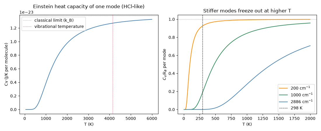
HCl vibrational temperature: 4152.3 K

At room temperature, HCl’s vibrational mode is still almost entirely frozen out (T << vibrational temperature), so it contributes almost nothing to the heat capacity – the classical equipartition expectation only becomes accurate at temperatures far higher than any real HCl gas would survive at:

Cv_room = hcl_mode.heat_capacity_v(298.15, N=1.0) / K_B
print(f"Cv_vib(298.15 K) / k_B = {Cv_room:.4f} (classical limit would be 1.0)")

plt.show()

Cv_vib(298.15 K) / k_B = 0.0002 (classical limit would be 1.0)