Gibbs’s canonical ensemble: all thermodynamics from one partition function

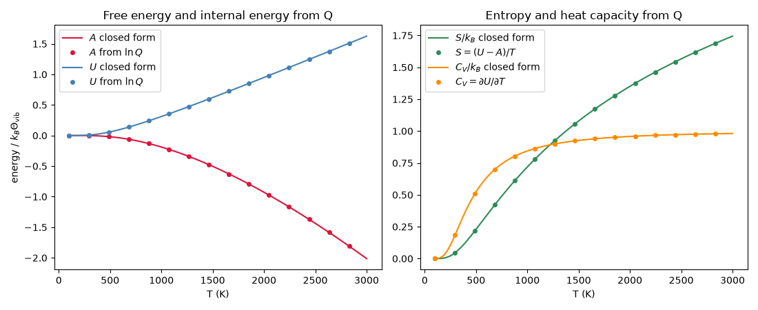
Gibbs (1902) showed that for a system at fixed temperature every thermodynamic function follows from the canonical partition function \(Q=\sum_i e^{-E_i/k_BT}\):

\[A=-k_BT\ln Q,\qquad U=k_BT^2\frac{\partial\ln Q}{\partial T},\qquad S=\frac{U-A}{T},\qquad C_V=\frac{\partial U}{\partial T}\]

Here the partition function of a vibrational mode is built by brute-force summation over its energy levels, and \(A\), \(U\), \(S\), \(C_V\) are obtained from it by nothing but differentiation. They agree with the closed forms of VibrationalPartitionFunctionHarmonic, and with helmholtz_free_energy() (\(A=U-TS\)). IdealGasMolecule then combines independent modes, whose partition functions multiply.

import matplotlib.pyplot as plt
import numpy as np

from chemistrykit.constants import K_B
from chemistrykit.statmech import IdealGasMolecule, VibrationalPartitionFunctionHarmonic

mode = VibrationalPartitionFunctionHarmonic.from_wavenumber(1000.0)
theta = mode.vibrational_temperature
levels = K_B * theta * np.arange(400)  # E_v = v h nu, measured from v = 0


def ln_Q(T):
    """Gibbs's sum over states, evaluated directly."""
    return np.log(np.sum(np.exp(-levels / (K_B * T))))


T = np.linspace(100.0, 3000.0, 120)
dT = 1e-2 * T
lnQ = np.array([ln_Q(t) for t in T])
dlnQ = np.array([(ln_Q(t + d) - ln_Q(t - d)) / (2 * d) for t, d in zip(T, dT)])

A = -K_B * T * lnQ
U = K_B * T**2 * dlnQ
S = (U - A) / T
Cv = np.gradient(U, T)

fig, axes = plt.subplots(1, 2, figsize=(11, 4.5))
for values, closed, label, color in [
    (A / (K_B * theta), mode.helmholtz_free_energy(T, N=1.0) / (K_B * theta), r"$A$", "crimson"),
    (U / (K_B * theta), mode.internal_energy(T, N=1.0) / (K_B * theta), r"$U$", "steelblue"),
]:
    axes[0].plot(T, closed, color=color, label=f"{label} closed form")
    axes[0].plot(T[::8], values[::8], "o", color=color, markersize=4, label=f"{label} from $\\ln Q$")
axes[0].set_xlabel("T (K)")
axes[0].set_ylabel(r"energy / $k_B\Theta_{\mathrm{vib}}$")
axes[0].set_title("Free energy and internal energy from Q")
axes[0].legend()

axes[1].plot(T, mode.entropy(T, N=1.0) / K_B, color="seagreen", label=r"$S/k_B$ closed form")
axes[1].plot(T[::8], S[::8] / K_B, "o", color="seagreen", markersize=4, label=r"$S = (U-A)/T$")
axes[1].plot(T, mode.heat_capacity_v(T, N=1.0) / K_B, color="darkorange", label=r"$C_V/k_B$ closed form")
axes[1].plot(T[::8], Cv[::8] / K_B, "o", color="darkorange", markersize=4, label=r"$C_V = \partial U/\partial T$")
axes[1].set_xlabel("T (K)")
axes[1].set_title("Entropy and heat capacity from Q")
axes[1].legend()
fig.tight_layout()

The same machinery applies to a whole molecule: for independent modes the partition function factorizes, so ln q and every derived function are sums over modes. thermodynamic_functions bundles them:

co2_like = IdealGasMolecule(mass=7.3e-26, volume=0.0248, moment_of_inertia=7.2e-46, symmetry_number=2, vibrational_frequencies=[4.0e13, 2.0e13, 2.0e13, 7.0e13])
tf = co2_like.thermodynamic_functions(298.15)
print(f"q = {tf.q:.3e}")
print(f"U = {tf.U:.1f} J/mol, S = {tf.S:.2f} J/(mol K), Cv = {tf.Cv:.2f} J/(mol K), A = U - TS = {tf.A:.1f} J/mol")
print(f"max |A_numeric - A_closed| / (k_B Theta) = {np.max(np.abs(A - mode.helmholtz_free_energy(T, N=1.0))) / (K_B * theta):.2e}")

plt.show()

q = 2.026e+33
U = 6888.0 J/mol, S = 213.81 J/(mol K), Cv = 28.83 J/(mol K), A = U - TS = -56858.0 J/mol
max |A_numeric - A_closed| / (k_B Theta) = 9.09e-16