Raoult’s law and the P-x-y diagram of an ideal solution

Raoult’s law, \(P_A = x_A P_A^*\) (raoult_vapor_pressure()), makes each partial vapor pressure a straight line in liquid mole fraction. Adding the two lines (Dalton’s law) gives the total pressure, and BinaryIdealSolution computes the vapor composition, which is always richer in the more volatile component. That enrichment is the basis of fractional distillation.

import matplotlib.pyplot as plt
import numpy as np

from chemistrykit.thermo.systems.mixtures import BinaryIdealSolution, raoult_vapor_pressure

P_benzene, P_toluene = 12.7, 3.8  # kPa, pure vapor pressures near 25 degC
solution = BinaryIdealSolution(P_A_star=P_benzene, P_B_star=P_toluene)
x = np.linspace(0.0, 1.0, 200)

fig, axes = plt.subplots(1, 2, figsize=(12, 4.8))
axes[0].plot(x, raoult_vapor_pressure(x, P_benzene), "--", label=r"benzene, $x_B P_B^*$")
axes[0].plot(x, raoult_vapor_pressure(1 - x, P_toluene), "--", label=r"toluene, $x_T P_T^*$")
axes[0].plot(x, solution.total_pressure(x), color="black", label="total")
axes[0].set_xlabel("liquid mole fraction benzene")
axes[0].set_ylabel("P (kPa)")
axes[0].set_title("Raoult's law: straight partial-pressure lines")
axes[0].legend()

axes[1].plot(x, solution.total_pressure(x), label="liquid (P-x, bubble line)")
axes[1].plot(solution.vapor_composition(x), solution.total_pressure(x), label="vapor (P-y, dew line)")
axes[1].set_xlabel("mole fraction benzene")
axes[1].set_ylabel("P (kPa)")
axes[1].set_title("P-x-y diagram for benzene/toluene")
axes[1].legend()
fig.tight_layout()

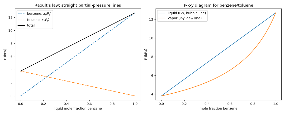
A 50:50 liquid gives a vapor much richer in benzene; condensing and re-evaporating repeats the enrichment (each step is one theoretical plate of a distillation column):

x_step = 0.5
for plate in range(1, 5):
    x_step = float(solution.vapor_composition(x_step))
    print(f"after plate {plate}: benzene mole fraction = {x_step:.3f}")

plt.show()

after plate 1: benzene mole fraction = 0.770
after plate 2: benzene mole fraction = 0.918
after plate 3: benzene mole fraction = 0.974
after plate 4: benzene mole fraction = 0.992