Hess’s law: reaction enthalpy does not depend on the path

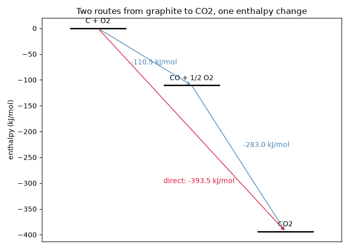
Burning graphite straight to \(CO_2\) releases the same heat as burning it first to \(CO\) and then burning the \(CO\). The enthalpy-level diagram below shows both routes, summed with hess_law_enthalpy(). The same principle lets reaction_enthalpy_from_formation() compute any reaction enthalpy from tabulated enthalpies of formation, shown here for the combustion of methane.

import matplotlib.pyplot as plt

from chemistrykit.thermo.systems.thermochemistry import hess_law_enthalpy, reaction_enthalpy_from_formation

dH_C_to_CO = -110.5  # C(graphite) + 1/2 O2 -> CO, kJ/mol
dH_CO_to_CO2 = -283.0  # CO + 1/2 O2 -> CO2
dH_direct = hess_law_enthalpy([1.0, 1.0], [dH_C_to_CO, dH_CO_to_CO2])

levels = {"C + O2": 0.0, "CO + 1/2 O2": dH_C_to_CO, "CO2": dH_direct}
fig, ax = plt.subplots(figsize=(7, 5))
for x, (label, H) in zip([0.0, 1.0, 2.0], levels.items()):
    ax.hlines(H, x - 0.3, x + 0.3, color="black", linewidth=2)
    ax.text(x, H + 10, label, ha="center")
ax.annotate("", xy=(1.0, dH_C_to_CO), xytext=(0.0, 0.0), arrowprops=dict(arrowstyle="->", color="steelblue"))
ax.annotate("", xy=(2.0, dH_direct), xytext=(1.0, dH_C_to_CO), arrowprops=dict(arrowstyle="->", color="steelblue"))
ax.annotate("", xy=(2.0, dH_direct), xytext=(0.0, 0.0), arrowprops=dict(arrowstyle="->", color="crimson"))
ax.text(0.35, -70, f"{dH_C_to_CO} kJ/mol", color="steelblue")
ax.text(1.55, -230, f"{dH_CO_to_CO2} kJ/mol", color="steelblue")
ax.text(0.7, -300, f"direct: {dH_direct} kJ/mol", color="crimson")
ax.set_xlim(-0.6, 2.6)
ax.set_xticks([])
ax.set_ylabel("enthalpy (kJ/mol)")
ax.set_title("Two routes from graphite to CO2, one enthalpy change")
fig.tight_layout()

Methane combustion, \(CH_4 + 2O_2 \to CO_2 + 2H_2O(l)\), from standard enthalpies of formation (kJ/mol):

dHf = {"CH4": -74.8, "O2": 0.0, "CO2": -393.5, "H2O(l)": -285.8}
dH_comb = reaction_enthalpy_from_formation([-1, -2, 1, 2], list(dHf.values()))
print(f"Two-step graphite combustion: {dH_direct:.1f} kJ/mol")
print(f"Methane combustion from formation enthalpies: {dH_comb:.1f} kJ/mol")

plt.show()

Two-step graphite combustion: -393.5 kJ/mol
Methane combustion from formation enthalpies: -890.3 kJ/mol